Showing posts with label Ice. Show all posts

Thursday, October 22, 2026

Antarctica’s Hidden Lakes Can Fill, Drain, and Move the Ice Above

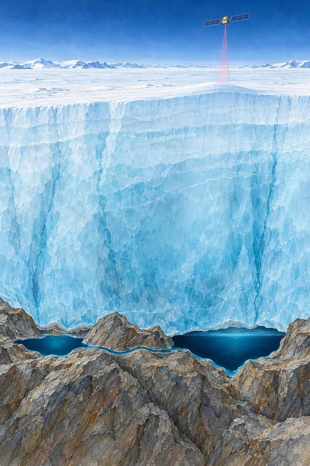
Painted cutaway of thick Antarctic ice above two liquid reservoirs connected along a rocky bed, with a satellite overhead.
Conceptual cutaway of basal lakes. Ice depth, lake shape, and satellite distance are compressed and are not observations of a named site.

Above an Antarctic lake, there may be no shoreline, no open water, and no visible basin. There may instead be a broad, almost featureless ice surface. Yet that surface can rise as water accumulates far beneath it, then sink as the hidden reservoir drains.

This is one way scientists study active subglacial lakes without drilling into every one. They measure changes in the top of the ice and work backward toward a hydraulic system at its base. The result is a continent with moving water hidden beneath an apparently frozen exterior.

Liquid water does not require a warm afternoon

At the base of an ice sheet, geothermal heat, friction, pressure, and insulation help determine whether water can remain liquid. It is misleading to picture every basal lake as surface melt that recently fell down a crack. The sources and connections vary with the glacial setting.

NASA’s early account of Antarctic subglacial lakes explains how interconnected reservoirs can fill and drain beneath fast-moving ice. Water follows hydraulic potential, which depends on pressure as well as bed elevation. A simple contour map of the bed cannot by itself tell the whole drainage story.

Imagine pressing down on a flexible water-filled bag resting on an uneven table. The water’s preferred route is influenced both by the table and by your applied pressure. This is only a conceptual analogy—the ice, sediment, and conduits are much more complicated—but it helps separate a subglacial system from an ordinary hillside stream.

The satellite measures the roof

Repeated altimetry compares the ice surface at different times. A localized rising or falling patch, with the appropriate spatial and temporal behavior, can indicate a filling or draining reservoir below. NASA’s 2021 ICESat-2 report describes improved measurements and the identification of additional active lakes.

The distinction between observation and inference matters. The laser does not pass through a kilometer of ice and bounce off the lake bottom. It measures the upper surface. Researchers must separate a basal-water signature from snowfall, ice dynamics, firn changes, and other processes that also alter that surface.

A useful figure should therefore show a time series, a footprint, and a surrounding comparison area. A single colorful depression is less informative than a repeated pattern of change supported by neighboring observations and an explanation of alternatives.

Three kinds of evidence to keep separate

What a hidden-lake claim can rest on
ObservationWhat it supportsWhat it does not show alone
Repeated localized surface uplift and subsidenceActive storage change beneath the iceA direct view of water chemistry or bed shape
Radar reflections compatible with a wet bedThe presence and geometry of a possible reservoirA complete filling-and-draining history
Direct clean-access samplingProperties of the sampled water and sedimentConditions in every other lake

These approaches can strengthen one another. Their conclusions still need to match their reach. An inventory of active lakes is not interchangeable with an inventory of every subglacial lake, because a stable reservoir may not produce a detectable surface cycle during the observation window.

A moving inventory, with dates attached

A 2025 study by Wilson and colleagues used a decade of CryoSat-2 observations to identify 85 previously unknown active lakes. The paper’s value goes beyond adding dots to a map: repeated cycles and connected groups reveal a changing hydrological system.

ESA’s account of that study gives a total of 231 known active lakes in that inventory. That is a dated research result, not a final count for all time. “Previously unknown” also means unknown to that observational inventory, not newly created in 2025.

This is a general lesson in discovery reporting. Improved spatial coverage, a longer time series, and a better detection method can change the number of known objects without the physical population suddenly increasing by the same amount.

Try a storage calculation

Suppose a hypothetical 20-square-kilometer patch rises by an average of one meter. Multiplying area by height gives 20 million cubic meters, or 0.02 cubic kilometers, of surface-volume change. This is a scale exercise, not a claim about a particular Antarctic lake.

Turning that change into an actual water-volume estimate requires a physical model. Ice can flex beyond the reservoir outline, the measured patch may not capture the full deformation, and other elevation processes must be removed. The arithmetic is useful because it shows both how a subtle height signal can represent substantial storage and why a surface measurement is not automatically a direct volumetric gauge.

For another comparison, imagine the same surface-volume change occurring over one month and over five years. The total storage change can be equal while the implied average transfer rates differ by a factor of sixty. A lake inventory without dates would hide that difference. This is why the timing of a fill-drain cycle is as scientifically useful as its footprint: geometry describes where the reservoir is, while the sequence reveals how the system operates.

Drainage can change more than the lake

Basal water influences the conditions under which ice moves. Its routing and pressure matter, so “more water means faster ice” is not an adequate rule for every situation. Efficient channels can behave differently from distributed, pressurized water storage.

ESA’s report on a major drainage event describes links between subglacial outflow, the grounding-zone environment, and ocean melting. Such results make the hidden plumbing relevant to ice-sheet evolution, while leaving substantial work in representing it in large-scale models.

The reader’s next step is to inspect a before-and-after elevation sequence rather than only a continent-wide map. Ask which lakes filled while another drained, whether their changes were simultaneous or delayed, and what uncertainty remains about the route between them. Antarctica’s apparent stillness then becomes a measurement challenge: the most revealing movement may be a small rise in a roof whose water is out of sight.

Sources and a next step

Continue exploring art, ideas, and unexpected connections at Incoprea.

Why Melting an Ice Sheet Can Lower the Sea Beside It

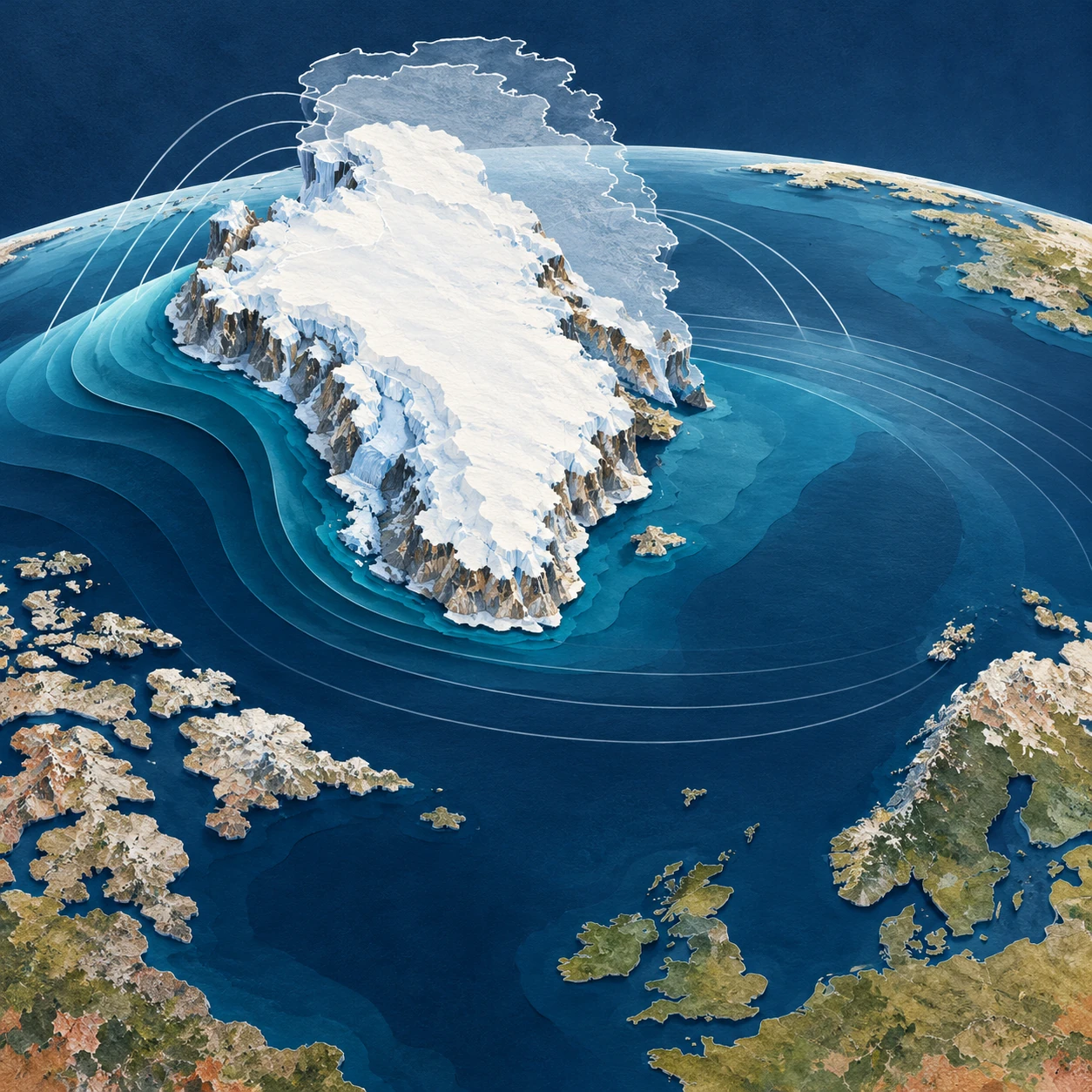
Conceptual cut-paper image of an ice-covered island and curved blue ocean layers with a faint outline of former larger ice.
Conceptual artwork of ice loss and ocean redistribution. Relief, coastlines, gravity arcs, and water-height differences are exaggerated and not a forecast.

Melting land ice adds water to the ocean. It seems obvious that the sea should rise everywhere. Yet close to a large ice sheet, one contribution to sea-level change can go in the opposite direction: the nearby sea can fall as the ice loses mass.

The apparent contradiction comes from imagining the ocean as a bathtub with a fixed bottom and a level surface independent of gravity. Earth has neither of those conveniences. Its sea surface, solid ground, and rotation all respond when a very large mass is moved.

An ice sheet attracts water

Greenland and Antarctica are not merely containers of frozen water. Their mass contributes to Earth’s gravitational field and attracts nearby ocean water. Remove some ice and that attraction weakens. Water redistributes away from the shrinking ice sheet, while the added meltwater is spread through the ocean in a geographically uneven way.

NASA JPL’s explanation of sea-level fingerprints describes why a source’s location and size create a characteristic response. A kilogram lost from one ice region does not have precisely the same local sea-level effect as a kilogram lost from another. The ocean retains information about where the mass came from.

“Attraction” here is not a second ocean sitting above the ordinary ocean. It is a small contribution to the shape of an already complex gravity-defined sea surface. The complete gravity field remains dominated by Earth as a whole.

The land is not a fixed ruler

Removing a load also allows solid Earth to deform, with both relatively rapid elastic responses and longer-lived adjustment to past ice changes. A coastline can move vertically while the ocean surface moves too. Relative sea level measures the water against the land at that location; satellite altimetry describes sea-surface height in a different reference system.

NASA’s sea-level FAQ places ice-mass redistribution alongside other reasons sea level differs geographically. Ocean circulation, heat, land-water storage, and local land motion further complicate the total observed change.

This is why a fingerprint is usually a statement about a particular contribution. A negative contribution from nearby ice loss does not guarantee that the total measured sea level at a particular harbor will be falling. Other terms can outweigh it.

Keep the accounting visible

Three different questions at the same coast
QuestionUseful quantity
What happens to the global water budget?Global mean contribution from land-ice mass loss
How is that contribution distributed?The source-specific sea-level fingerprint
What happens to this shoreline?Total relative sea level, including land motion and other ocean effects

Confusing these questions makes good science sound contradictory. A global average can rise while a component falls locally. A tide gauge can show a different trend from the neighboring sea surface if the ground carrying the gauge is moving.

A thought experiment with two islands

Imagine two coastal communities, one near a large ice sheet and one far away. Transfer the same amount of ice mass into the ocean in two hypothetical worlds: first from the nearby sheet, then from a distant sheet. Keep other factors fixed for the exercise.

The global mean added-water contribution could be the same in both worlds, while the local outcomes differ. In the first world, the nearby community experiences reduced attraction and a local solid-Earth response associated with its neighboring sheet. In the second, it occupies a different part of the distant source’s fingerprint.

No numerical forecast follows from this sketch. To calculate the difference, scientists need the geography of ice loss and a model that includes the relevant gravitational, rotational, and deformational response. The thought experiment simply shows why knowing the total melt is insufficient for knowing every coast’s change.

In your two-island sketch, use separate arrows for added water, changed attraction, and moving land. Do not draw one combined arrow until each contribution has a sign. This simple bookkeeping prevents the counterintuitive local response from obscuring the global mass balance that remains true at the same time.

How do scientists test the pattern?

One route combines gravity observations, estimates of land-water and ice-mass changes, and ocean measurements. NASA’s 2017 report of detected fingerprints describes evidence in ocean observations for predicted geographical patterns associated with changing continental water storage and ice mass.

Detecting the pattern is difficult because it sits within ocean variability rather than appearing as a neat ring on the sea. A model fingerprint is a structured prediction to test against data, not a colored map that becomes true merely because it was calculated.

A NASA modeling account shows how ice dynamics and sea-level response can be linked. Such coupled work is especially useful when the spatial pattern of mass loss changes over time instead of remaining one fixed source.

Read a fingerprint map carefully

Before interpreting its colors, find the normalization. Some maps show actual projected changes under a scenario; others show a response per unit of global mean sea-level contribution. A value on the second kind of map is a multiplier, not automatically a number of centimeters.

Then check whether the map includes only one source of ice loss, whether it is relative to land, and what time span or Earth model it assumes. A striking blue region near Greenland may mean a negative contribution from Greenland’s own loss. It does not erase storm surge, waves, subsidence, or the contributions of other ice sheets.

JPL’s work linking port-city sea level to regional ice melt illustrates why the source geography matters for place-specific assessment. The point is a more complete accounting of risk, not a promise that a nearby ice sheet protects every northern coast.

The useful surprise is that “level” is a physical condition rather than a universal height. Move enough mass and the meaning of the ocean’s resting surface changes. Once that is understood, the local fall beside melting ice stops being a paradox and becomes a measurable part of the larger rise.

Sources and a next step

Continue exploring art, ideas, and unexpected connections at Incoprea.
The Elevator With Three Working Buttons

Case 50 · shortest-path challenge · Hard · About 10-15 minutes The archive elevator has a peculiar test mode. Its floor display works, but o...