Showing posts with label Water. Show all posts

Sunday, October 25, 2026

A Water Strider Rows the Shape of the Pond

Watch a water strider from the bank of a still pond and its legs seem to rest on invisible supports. Look more closely and the supports become visible as dimples. Each long leg presses the surface downward without ordinarily breaking through it. The insect is not standing on a solid skin. It is reshaping an interface, and that shape helps carry its weight.

A water strider above surface dimples, with stylized swirls depicting water motion beneath it.
Surface dimples and an imagined view of the water moving beneath a strider’s legs.

Begin with the dimple, not the insect

Surface tension acts along the air–water boundary. When a non-wetting leg depresses that boundary, the curved surface provides an upward contribution to support. The leg’s length spreads contact across a substantial distance relative to the insect’s body. The classic hydrodynamics study describes weight support through the curved free surface and propulsion through the middle pair of legs. It is useful to separate those two tasks: staying up and moving forward are related, but they are not the same question.

The phrase “water has a skin” is convenient until it starts suggesting a sheet of rubber with fixed edges. Water flows, and its surface changes continuously. A strider must create forces through contact with that moving boundary. If you imagine a rigid platform under each foot, you lose the central feature of the problem: the platform itself is made by the foot and disappears when the foot moves away.

Its legs also have a specialized surface. Gao and Jiang examined the non-wetting legs of a water strider and emphasized their tiny oriented hairs and finer grooves. This hierarchical structure helps resist wetting, rather than leaving the explanation solely to wax chemistry. Their 2004 paper connects a feature visible in a pond with features requiring much greater magnification. A dry-looking foot is the outcome of both geometry and material behavior.

The wake below the apparent surface

How can a stroke against water generate forward movement? Earlier explanations emphasized waves traveling away from the insect. That raised a difficulty: very young striders can move even when their legs are too slow to generate the relevant waves. Hu, Chan, and Bush used high-speed video and particle tracking to reveal another route. Their experiments showed that driving legs transfer momentum into vortices in the water below, resolving the apparent contradiction.

In ordinary language, a rowing stroke gives some surrounding water backward momentum while the animal gains forward momentum. Surface ripples may still occur; the finding was that capillary waves were not the primary momentum pathway in the measured locomotion. That distinction is more precise than claiming the insect makes “no waves.” The visible rings can draw our attention away from a less visible, dynamically important wake underneath.

A later fluid-mechanics analysis explored these flows in greater detail. Such work turns a charming observation into a testable balance: what forces act, how long do they act, and where does the transferred momentum go? An animal’s speed is only one part of the evidence. Tracking the water lets researchers test an explanation instead of judging it by the insect’s movement alone.

Jumping asks a different question

Some water striders can also launch themselves upward. Here, pushing harder is not automatically better. A stroke that breaks the surface too early changes the available support. In a 2015 study of jumping insects and robots, researchers found that curved leg tips rotated inward while the legs pushed down at a controlled speed. The movement kept the applied force below the threshold that would break the surface under those conditions.

A later comparative study examined how striders adjust leg speed in relation to body form. Its importance lies in the match between a movement and its supporting surface. A pond does not offer the same resistance as a stone. The best push depends on the animal’s mass, leg geometry, and the behavior of the interface, so a rule taken from one body size or species should not become a slogan about every water-walking insect.

If you film from the bank, use the ordinary recording as a record of visible behavior, not a laboratory measurement of forces. Reflections can hide a leg, surface breezes can create unrelated ripples, and a camera angle can compress a backward stroke into an apparent sideways movement. Writing down those uncertainties often makes the observation more interesting. It gives you specific things to look for on a second visit.

The larger lesson is about where to search for a mechanism. A strider’s secret is neither wholly inside its body nor wholly in a remarkable coating. It emerges from an interaction among leg structure, timing, surface shape, and the water’s response. The pond is part of the locomotor system. Once you notice that partnership, a few delicate dimples become evidence of an animal continually building the surface it moves across.

Sources and further exploration

Two more connections

Visit Incoprea

A Bell Siphon Turns a Steady Inflow Into a Repeating Flood

Water enters a growing bed at a steady rate. For several minutes the level rises quietly. Then the drain begins to run much faster, the bed empties, a gulp of air interrupts the flow, and filling starts again. No clock has counted down to either transition.

A bell siphon can create this flood-and-drain cycle through the arrangement of water, air and pipes. Its useful feature is the change between two modes. At the same intermediate water level, the bed can be filling on one part of the cycle and draining on another.

Simplified transparent bell-siphon model with an upper tank, capped bell and standpipe draining toward a lower tank.
The bell encloses the standpipe so rising water can start a full siphon and falling water can later admit air.

Meet the standpipe and its cover

The standpipe is a vertical drain rising from the bed's floor. Uncovered, it behaves as an overflow: water reaching its top can spill into the pipe and leave. Once the level falls below that opening, ordinary overflow stops.

The bell is a wider capped cover placed around the standpipe. Water enters beneath its lower edge or through openings near its base. The enclosed space lets the system change from a trickling overflow to a full siphoning flow as water rises and air is displaced.

During a successful start, water fills the drain sufficiently to establish the siphon. The descending outlet lies lower than the bed's water surface. Gravity supplies the energy for flow through the connected water path, while pressure differences help draw water up beneath the bell and over the standpipe.

Once established, the flow can continue after the bed's level has fallen below the standpipe's top. Water still reaches the siphon's intake near the bell's bottom. That extension below the overflow level is what allows the bed to drain substantially.

Stopping is part of working

As the level drops toward the lower inlet, air can enter the bell. Some designs add a snorkel tube to admit air at a chosen low level. Enough air breaks the continuous siphoning condition, and the fast drainage ends.

The continuing inlet can then refill the bed. A working cycle needs both transitions: overflow must develop into a siphon, and the siphon must later admit enough air to stop. A device that drains vigorously but never resets has completed only half the task.

The University of Hawai‘i's original bell-siphon publication includes component photographs and its described start-and-break sequence. Use those photographs to identify the capped bell, standpipe, low openings and snorkel. These features have different jobs; an outer gravel guard, for example, keeps growing media away without creating the siphon itself.

Read a cycle as a water account

Consider an invented clear tank with a straight-sided shape. Between its low and high switching levels it stores 12 litres. Water enters at 2 litres per minute. During the draining phase, suppose the total outlet flow stays at 8 litres per minute.

These are deliberately simplified, constant rates for a calculation. Real siphon flow changes with water level and geometry. The exercise concerns the difference between outlet flow and the rate at which the tank's contents decrease.

A hypothetical cycle with continuous inflow
PhaseInflowOutflowNet change in stored water
Filling2 litres/minuteAssumed zeroGain of 2 litres/minute
Draining2 litres/minute8 litres/minuteLoss of 6 litres/minute

How long would each phase take under those assumptions? Include the incoming water during drainage before checking the answer.

Work through the timings

Filling 12 litres at 2 litres per minute takes 6 minutes. Draining the same stored difference at a net loss of 6 litres per minute takes 2 minutes. The idealised cycle lasts 8 minutes. During drainage, 16 litres leave: the initial 12 litres plus 4 more that arrive during those 2 minutes.

If you had divided 12 by 8 for the draining time, you would have counted the outlet while forgetting the continuing inlet. The error is small enough to look plausible and large enough to change your picture of the cycle.

A level can remember which way it was going

Choose a water level halfway between the two switching heights. On the way up, the drain may not yet have established its full siphon. On the way down, the siphon is already running. The same depth can therefore accompany different outlet flows.

This dependence on the preceding state gives the system a simple kind of memory. The apparatus needs no stored number saying “drain now.” Whether the pipe is filled for siphoning, and whether air has re-entered, provides the relevant physical state.

It also explains why looking at water height alone can be misleading. A short video showing the direction of change supplies information that one photograph lacks. To understand a complete mechanism, follow one full rise, transition, fall and reset.

The growing bed is part of the timing

In a media-filled bed, gravel or expanded clay occupies some of the apparent tank volume. Water fills the connected spaces around that material. A depth change therefore cannot be converted into litres using the empty container's dimensions alone.

Virginia Cooperative Extension's overview of media hydroponic systems places standpipes and bell siphons within recirculating arrangements. It describes nutrient solution being pumped from a lower reservoir to a planted container, then returning after flooding.

The siphon controls a return flow; the separate pump that raises water to the bed still requires energy. Substrate, roots and accumulated material can also change available flow paths. A working bell does not make the surrounding growing system independent of maintenance or water management.

The most revealing moment is the gulp at the end. Air, often treated as an obstacle to liquid flow, has become the reset signal. A steady supply can produce a repeating rhythm because the water path changes state, then changes back.

Sources and further reading

Explore more art, stories and discoveries at Incoprea.

The Pump That Sends Water Uphill by Letting Most of It Fall

A pipe delivers water downhill to a small metal machine beside a stream. The machine clicks repeatedly. Another pipe carries water uphill, apparently without a motor. Look closer and the missing part of the story appears beside it: much of the incoming water is pouring back out.

This is a hydraulic ram pump. Its useful trick is to trade a large quantity of water falling a modest distance for a smaller quantity rising farther. The waste outlet is central to the explanation. Watching only the delivery pipe makes an ordinary energy conversion look like an exception to gravity.

Illustration of a hydraulic ram pump beside a stream, with discharge water returning to a channel.
A ram pump raises part of a falling water supply while the rest leaves through its waste outlet.

Give the machine three addresses

Imagine three levels: the source above the pump, the pump itself, and a storage tank higher still. The vertical drop from source to pump supplies the energy. The vertical rise from pump to tank is the task that energy must accomplish.

The lengths of the pipes are different quantities. A long pipe following a gentle slope may connect two points with little difference in elevation. That arrangement has less gravitational energy available per litre than a short, steep descent with a larger vertical drop.

University of Missouri Extension's discussion of livestock watering places the ram among pumping options that depend on the site's energy resources. It requires an appropriate downhill supply and uses considerably more drive water than it delivers. A level pond beside a hill does not provide the same opportunity merely because it contains plenty of water.

Listen for the interruption

The repeating cycle begins with water moving through the drive pipe and escaping through an open waste valve. As flow builds, the valve closes. Moving water cannot lose its momentum everywhere along the pipe instantaneously. A pressure disturbance travels through the water and pipe: water hammer.

That pressure pulse opens a delivery valve long enough to admit some water toward the delivery side. A conventional ram includes an air chamber. Compressing its trapped air stores some energy and helps smooth the pulsed supply into a more continuous delivery.

As the pressure changes, the delivery valve closes against return flow and the waste valve opens for another cycle. NC State Extension's component drawing is a useful way to follow the two valves separately. One releases drive water; the other helps keep delivered water from simply returning.

The rhythm is therefore a sequence of changing conditions, rather than a permanently open shortcut uphill. The supply repeatedly accelerates, encounters a restriction and transfers part of its energy. The chamber and valves allow those short events to serve a sustained task.

Keep two accounts: water and energy

Here is an invented example for reasoning, not a pump specification. Suppose 10 litres per minute enter a ram with a 2-metre fall. The tank is 10 metres above the pump. Assume that half the available drive-water energy becomes useful elevation energy in the delivered water.

The approximate balance is: delivered flow equals incoming flow, multiplied by fall, multiplied by efficiency, divided by lift. With our assumptions, that is 10 × 2 × 0.5 ÷ 10, or 1 litre per minute. The remaining 9 litres per minute leave through the waste route.

One hypothetical minute of operation
QuantityValueWhat it tells us
Incoming water10 litresThe whole drive supply
Delivered water1 litreThe useful raised fraction
Waste discharge9 litresWater returning at the pump's lower level
Assumed energy efficiency50 percentNot the percentage of water delivered

The last row matters. Delivering one tenth of the incoming volume does not mean the energy efficiency is one tenth. That smaller volume reaches a greater elevation. British Columbia's agricultural factsheet sets out this energy balance and treats performance as dependent on the relationship between fall and lift.

Your turn: move the tank

Keep the same incoming flow, fall and hypothetical efficiency, but raise the tank to 20 metres above the pump. Predict the delivered flow before opening the answer.

See the calculation

The estimate becomes 10 × 2 × 0.5 ÷ 20 = 0.5 litres per minute. Doubling the lift halves the delivered flow in this simplified comparison. Actual efficiency and pipe losses can change with operating conditions, so this is an energy-budget exercise rather than a performance guarantee.

Now compare the continuous rate with a daily total. One litre per minute becomes 1,440 litres over 24 hours, if the assumed supply and operation persist. A modest flow can accumulate into a useful reserve. A large-looking discharge may still deliver too little if the source weakens seasonally.

Returning waste water to the stream preserves its presence downstream, but it does not erase the consequences of diverting it through the machine. The stream reach between intake and outlet, available seasonal flow, sediment and the receiving channel all remain part of the setting.

A ram's appeal is clearest when the whole landscape stays in view: source, descent, waste route and destination. The clicking machine is the meeting point of those conditions. It turns an available fall into a useful rise, one small transfer at a time.

Sources and further reading

Explore more art, stories and discoveries at Incoprea.

Saturday, October 24, 2026

Rain Gives a Combined Sewer a Second Job

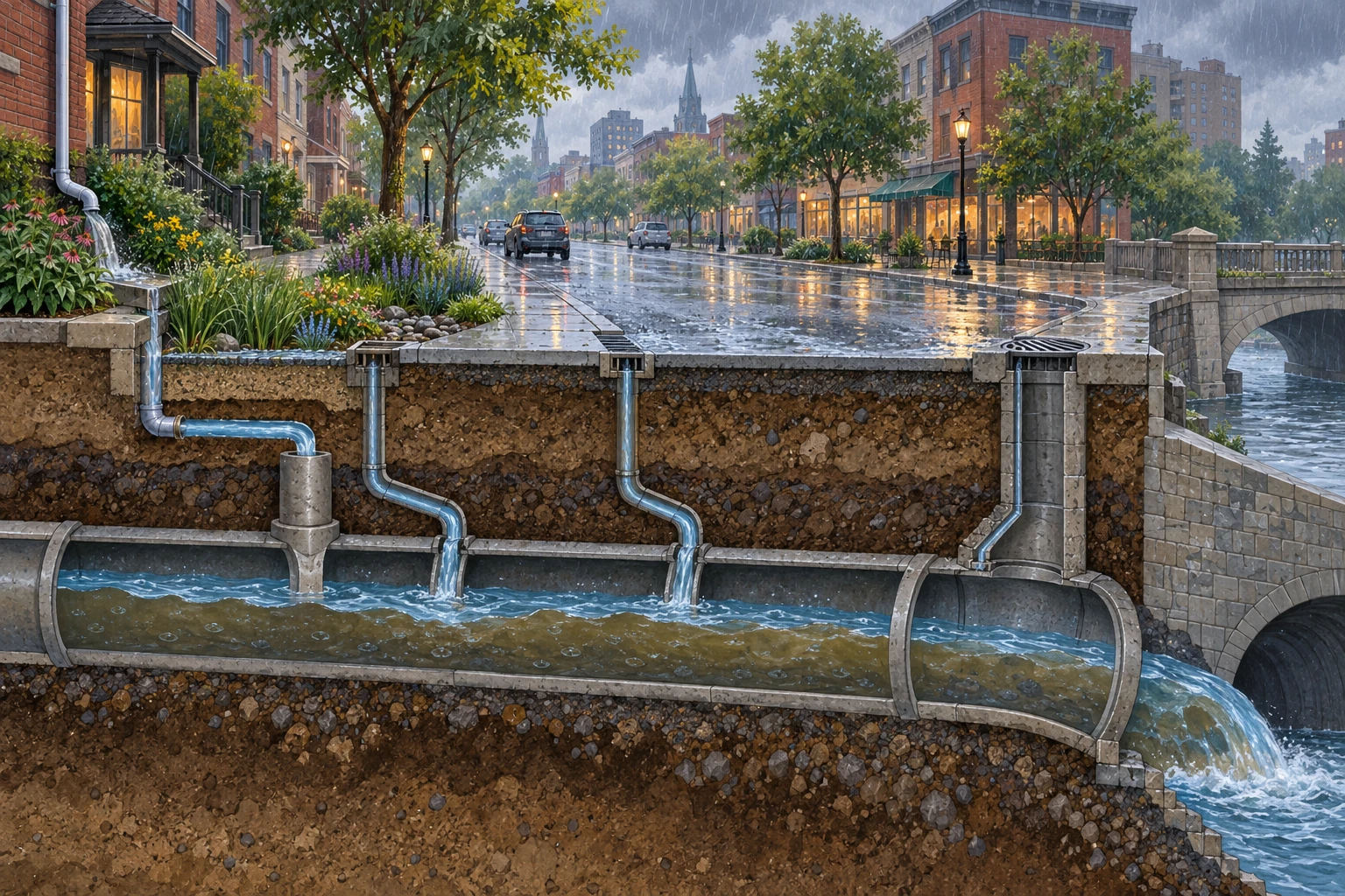
Rain begins on a city block. Water slides off roofs, runs along gutters and disappears through grates. Below the street, another flow was already present: the wastewater leaving buildings. In a combined sewer, the two meet.

The pipe has acquired a second job without receiving a second diameter. The interesting question is not simply whether rainwater looks clean at the curb. It is how the extra flow changes the work of a network already carrying wastewater toward treatment.

A conceptual street cutaway shows rain runoff entering a large shared underground pipe.
The cutaway emphasizes added runoff. It omits a real system’s regulator and treatment route and is not a complete sewer layout.

Follow the shared route

EPA’s combined-sewer explanation distinguishes a system carrying wastewater and stormwater together from separate sewer arrangements. During wet weather, the flow can exceed what the system or treatment facility can handle. Combined sewer overflows can then release a mixture that includes untreated wastewater into receiving waters.

That mixture matters. Rain may dilute some concentrations, but dilution is not the same as eliminating contaminants or treating sewage. A discharge’s environmental effect depends on more than the amount of water in the pipe.

The illustration emphasizes runoff entering a shared conduit. It omits the regulator and treatment route, so it should not be used as a complete plumbing diagram. In a real city, maps and operator documentation establish which drains connect to which system.

A large tank buys time, not infinity

Use a fictional constant-flow example. Background wastewater arrives at 50 litres per second. The outgoing route can handle 150 litres per second. A storm adds 200 litres per second, giving a total inflow of 250. The excess rate is therefore 100 litres per second.

Ten thousand litres of initially empty spare storage can hold that excess for 100 seconds. After two minutes, the event has produced 12,000 litres of excess. The storage holds 10,000, leaving 2,000 beyond its capacity. These are invented teaching values, not a description of any city’s sewer.

When does temporary storage run out?

A transparent constant-flow budget separates incoming runoff, treatment capacity and spare storage.

Open when does temporary storage run out? in its own window.

Reduce the rain inflow to 100 litres per second. Combined with the background 50, the total equals the assumed outgoing capacity. In this ideal constant-flow model there is no excess to store. Then set rain inflow back to 200 and double the duration. The same peak now creates much more total excess.

Notice the assumptions behind the hundred-second answer. Storage begins empty, the added flow is constant and the outgoing capacity remains available. A partly full tank or a changing downstream condition would produce a different result. Reading those assumptions is as important as checking the subtraction, because real storms rarely behave like a flat input line.

Volume and timing are different levers

A storage tank can temporarily hold water and release it when capacity becomes available. A surface that keeps runoff from reaching the combined network can reduce the input. A measure that delays runoff may help with a peak while leaving a different total volume over a longer interval.

EPA’s guidance on green infrastructure and CSO control treats such measures as components of broader planning. A planted area is not automatically a complete solution. Location, soils, available space, maintenance and the actual network all affect the role it can play.

For a paper exercise, draw three columns: avoid entering the pipe, hold temporarily and increase conveyance or treatment capability. Put a rain garden, a storage tank and an expanded facility into the columns they most directly affect. Some projects touch more than one job. The exercise helps you ask what a proposal changes instead of sorting solutions by whether they look green or grey.

The city is not one uniform pipe

New York City’s Department of Environmental Protection explains its combined-system context and the relation between runoff and overflow. A city-level explanation can still contain neighborhoods with different arrangements. “This city has combined sewers” does not establish the connection of every individual grate.

A reader investigating locally can begin with the water authority’s system map, overflow information and public project descriptions. Look for the distinction between a combined overflow and a separate sanitary-sewer failure. Similar-looking water at an outfall can belong to different mechanisms and responsibilities.

Read a stormwater proposal with three questions

What flow or volume is the project designed to change? Under which storm assumptions was it modeled? What happens when the planned storage fills or the input exceeds those assumptions?

Then ask how the project will be maintained and how actual performance will be observed. A model describes conditions and rules. Monitoring tests whether the real system behaves as expected. Neither an attractive rendering nor a single dramatic storm photograph can answer all of those questions.

The underground pipe becomes easier to understand when rain is treated as a timed input rather than background scenery. A city manages not only where water goes, but how much arrives together and what room remains when it gets there.

Sources and further exploration: EPA: combined sewer overflow basics; EPA: green infrastructure in CSO control; New York City DEP: combined sewer overflows.

Explore all 50 new articles · Browse the complete illustrated collection

Explore more art, ideas, and independent projects at Incoprea.

The Venetian Wellhead Is Only the Handle of a Larger Water Machine

A stone wellhead stands in a Venetian square like an elaborate piece of furniture. Its opening is modest, its carved sides weathered, its silhouette easy to photograph. The tempting assumption is that a simple shaft descends to a convenient underground supply of fresh water.

The larger historical system asks you to look sideways. The wellhead was the visible access point to a rainwater-collection arrangement extending beneath the surrounding surface. The square could participate in supplying water, not merely decorate the place where it was drawn.

A weathered stone wellhead stands on wet paving in a Venetian square.
The visible wellhead is an access point. The collection and storage arrangement extends beneath the surrounding surface.

Separate the opening from the reservoir

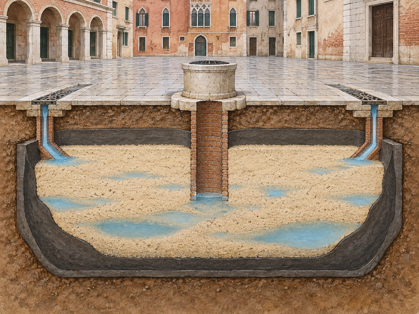
The City of Venice’s account of its freshwater supply describes rain directed from roofs or prepared surfaces into filtering cisterns. Layers of sand and a surrounding clay barrier helped separate the collected freshwater from the brackish environment. The stone vera da pozzo covered and protected the access shaft.

That arrangement changes the object you are looking at. The narrow central opening does not tell you the footprint of the surrounding storage structure. Nor does the depth of a visible wellhead reveal how much usable water its whole system could provide.

Imagine a tree whose trunk is all you can see above the soil. It would be a mistake to infer the entire underground extent from the trunk’s width. The analogy is limited—cisterns are built structures, not roots—but it prompts the right change of attention.

A conceptual cutaway shows a central brick shaft inside a sand-filled clay-lined basin below a square.
A simplified section separates access shaft, sand and water barrier. It supplies no surveyed dimensions or measured storage volume.

Water can occupy a structure filled with sand

A sand-filled basin may seem to leave no room for storage. Yet grains do not pack without gaps. Water can occupy connected spaces between them. The amount depends on the material and geometry; the cutaway is conceptual and supplies no measured pore fraction.

Beltrame and colleagues’ archaeological research examines well-cisterns in the Venice Lagoon and the northeastern Adriatic. Their work places water collection within a landscape of navigation and changing settlement. A familiar architectural feature can therefore connect to a much longer and more varied history than the decorative wellhead alone suggests.

Keep filtration separate from a modern guarantee of potable water. The historical purpose of a system and its ability to remove particular contaminants are different questions. An appealing diagram of sand does not establish that collected water is safe to drink.

Try a budget before admiring the tank

Suppose a fictional collection surface covers 100 square metres. A 20-millimetre rain event places 2,000 litres on that area. If an assumed 80 percent reaches storage after losses, the input is 1,600 litres. Those values illustrate units, not a measured Venetian installation.

How much rain reaches a cistern?

A unit-aware one-event water budget separates rainfall volume, collection losses and storage capacity.

Open how much rain reaches a cistern? in its own window.

Now reduce the usable capacity to 1,000 litres. The same rain can deliver 1,600 litres, but the initially empty store retains only 1,000. Increasing the catchment does not remove that bottleneck. In a second scenario, give the tank ample capacity and remove the rain. A splendid reservoir cannot collect water that never arrives.

This small calculation separates three constraints: the area collecting rain, the fraction that reaches storage and the volume available to hold it. Actual operation also depends on demand and timing. A yearly rainfall total cannot tell you how long water remains available through a particular dry interval.

The weather was not the only supplier

The city’s account also describes freshwater brought from the Brenta by boats. Storage and transport complemented local rain collection. Reading the system as a perfectly self-contained rain machine would leave out that logistical work.

Ferrara’s municipal explanation of cisterns “alla Veneziana” documents the same broader architectural tradition outside Venice. Its Palazzo Paradiso example includes a sand-filled basin and connected cisterns. The label identifies an approach that could be adapted, rather than one universal underground layout.

Read a square as infrastructure

In a photograph, locate the wellhead, any visible rain inlets and the slopes or joints of the surrounding paving. Mark features you can see with solid lines and inferred connections with dotted ones. Do not turn a possible drain into a proven cistern inlet without documentation.

Then list the invisible jobs: maintaining a water barrier, keeping collection surfaces usable, clearing inlets and managing supply during dry periods. Infrastructure includes care over time, even when its most memorable public object is stone.

The next wellhead you notice can become the start of a larger question. Where did the water come from, how was it protected, and how did people keep it available? The small opening is an invitation to imagine the whole square working.

Sources and further exploration: City of Venice: Rio dell’acqua dolce; Beltrame and colleagues: Roman well-cisterns; City of Ferrara: cisterns alla Veneziana.

Explore all 50 new articles · Browse the complete illustrated collection

Explore more art, ideas, and independent projects at Incoprea.

The Staircase That Follows the Water Underground

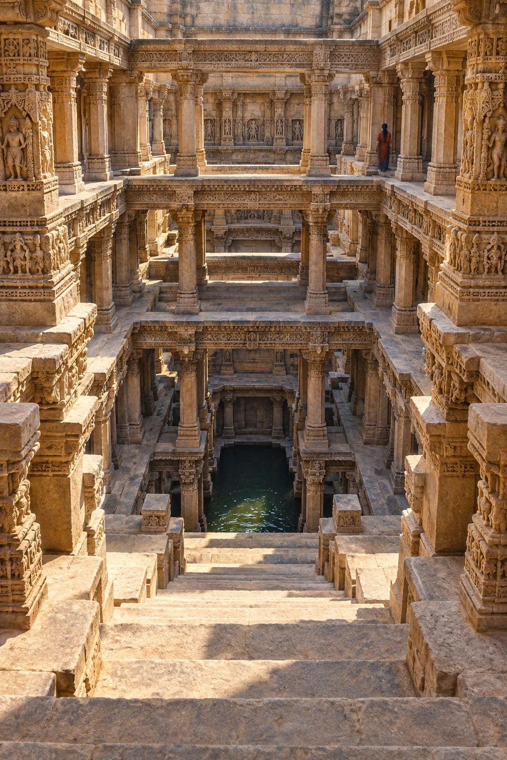
Most buildings invite us to look upward. A stepwell interrupts that habit. At ground level there may be an opening in a comparatively flat landscape; beyond it, stairs carry the eye down through repeated columns, landings and shadow. The important destination is below the street.

The geometry serves a practical challenge. A water surface need not remain at one height. A descending route can provide access at different levels, making the journey to water part of the building rather than leaving the entire task to a bucket dropped from above.

A deep sandstone stepwell descends through carved columns and landings toward dark water.
An architectural interpretation inspired by Indian stepwells. It is not a surveyed view of Rani-ki-Vav or Adalaj.

Read a section before a façade

Picture a simple well as a shaft. Now add a corridor that slopes down by a series of steps. The shaft and corridor perform different jobs: one reaches water; the other admits people toward it. Add landings and supporting structures, and the descent becomes a succession of spaces rather than one uninterrupted stair.

UNESCO’s account of Rani-ki-Vav at Patan describes an east–west composition with a stepped corridor, pavilions, a tank and a well shaft. Built in the eleventh century as a memorial, the monument combines water architecture with a religious conception of an inverted temple. Its seven levels do not reduce to seven interchangeable storage shelves.

The difference between a building’s plan and its section is especially vivid here. A plan can show where a corridor runs. A section reveals how shade, access and depth are organized. When looking at photographs, try tracing both the horizontal route and the vertical descent.

A changing level changes the journey

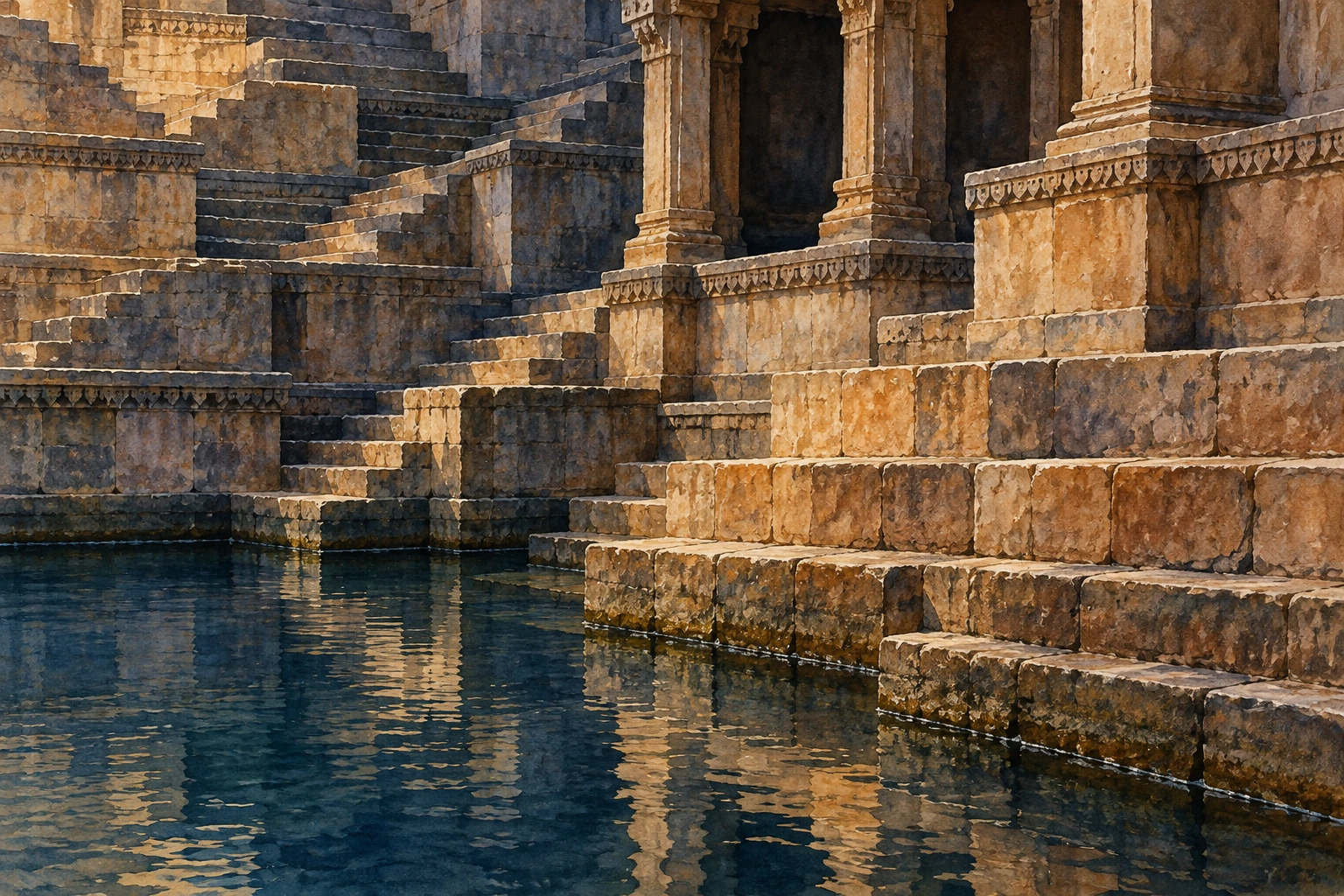
Imagine a harmless paper model: draw a staircase on a vertical sheet, then place a horizontal strip of blue paper across the lower steps. Slide the strip downward. More stairs emerge, and the point where a person reaches the water moves farther from the surface.

This is a geometric exercise, not a hydrological simulation. It does not predict how fast an aquifer falls or how a particular well refills. Its value is to make one design relationship visible: access can be distributed through height.

Stone stairs meet a dark water surface beneath a carved pavilion.
Follow the point where the stairs meet the water. A different level would change how far down someone must go.

Now add three landings to your drawing. Ask where two people could pass, where a vessel could be set down and where someone might pause. Those questions reveal how a water structure can also become a social space. They are questions to investigate in a real site’s evidence, rather than proof that every landing had one fixed purpose.

The stone is doing more than holding back earth

Gujarat Tourism’s Rani-ki-Vav record draws attention to the sculptural richness and the monument’s association with Queen Udayamati. Looking only at its hydraulic function would miss the commissioned, commemorative and sacred dimensions of the descent.

A useful close-looking task is to choose one photograph and temporarily ignore the water. Find a repeated structural element, then a variation: a carved figure, a change of opening or a band of ornament. Repetition gives your eye a rhythm. Variation tells you that this is a composed cultural environment, not merely a hole with efficient stairs.

Do the opposite on a second pass. Ignore ornament and follow the loads. Which horizontal elements span openings? Where do columns continue downward? A visitor does not need to solve the engineering to notice that sculpture and structure occupy the same carefully organized space.

There is more than one stepwell story

The Ahmedabad district record for Adalaj Vav offers another monument to examine. Comparing named examples is more revealing than treating all Indian stepwells as copies of a single photograph. Their plans, patronage, carving and settings deserve individual attention.

Try comparing just three features: the shape of the entry, the pattern of openings and the relationship between open sky and enclosed space. Write down what is visibly different before searching for a broad explanation. “Stepwell” identifies a family of water architecture, not a promise that every member has identical geometry or use.

A dry monument can still explain a water system

UNESCO notes that Rani-ki-Vav no longer functions as a water well following changes affecting the Saraswati riverbed and groundwater conditions. A present-day photograph of a dry lower space therefore cannot establish its historical operating water level.

When studying any heritage structure, separate three things in your notes: what survives now, what documentary or archaeological evidence establishes about the past, and what your imagination fills in. The illustrations here are interpretations of the architectural idea, not survey drawings of a particular monument.

A stepwell makes an ordinary necessity spatially extraordinary. Instead of hiding the distance to water, it gives that distance stairs, pauses, columns and meaning. Looking downward becomes a way to see how a community built around a resource that could move.

Sources and further exploration: UNESCO: Rani-ki-Vav; Gujarat Tourism: Rani Ki Vav; Ahmedabad district: Adalaj Vav.

Explore all 50 new articles · Browse the complete illustrated collection

Explore more art, ideas, and independent projects at Incoprea.

Friday, October 23, 2026

Ringwoodite: The Water Held Inside a Mantle Mineral

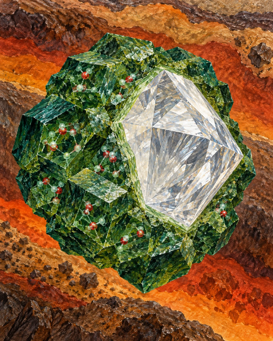
A small brown diamond contained a mineral grain too small to admire without instruments. That grain mattered because its crystal structure and infrared signature offered a physical sample of conditions far deeper than ordinary drilling can reach.

In 2014, researchers reported hydrous ringwoodite enclosed in a diamond from Juína, Brazil. Ringwoodite is a high-pressure form of the mineral olivine. Its relevance to water comes from hydrogen that can be incorporated into its structure, commonly described in terms of hydroxyl groups.

A conceptual arrangement places a diamond-like host, green mineral forms and molecular motifs against deep-Earth colors.
The mineral and diamond forms are arranged to explain a chemical relationship, not the actual geometry of the recovered inclusion. Molecular marks are symbolic and do not show measured bonding or free liquid.

“Water content” needs a chemical translation

A mineral’s reported water content need not mean that liquid water fills visible pores. For ringwoodite, hydrogen can occupy defects in the solid’s structure. Reporting the equivalent amount of H₂O is a convenient compositional accounting convention.

The Northwestern account of deep-water research explains this hydroxyl form and emphasizes the remaining question of extent and heterogeneity. The attractive image of a deep reservoir should not make a solid mineral into an open chamber of liquid.

That distinction does not make the reservoir trivial. A small mass fraction multiplied by a vast amount of rock can represent a large amount of hydrogen and oxygen. It simply changes what is being stored and how it can move.

What the diamond established

Pearson and colleagues’ primary paper used X-ray diffraction and Raman and infrared spectroscopy to identify the inclusion and its hydrous character. The result supplied direct evidence that at least part of the mantle transition zone contains water-bearing mineral material.

The transition zone is usually discussed as the mantle region between roughly 410 and 660 kilometres deep. Ringwoodite is stable within a portion of that range. A single recovered inclusion is powerful evidence of local conditions, but it is not a sample of every part of the shell.

The University of Alberta’s account of the discovery describes the analytical work required to find and characterize the tiny grain. Its crucial point is the existence of a local hydrous sample. Extrapolating from that sample to a total mantle inventory requires additional assumptions.

Do the multiplication, then inspect its assumptions

Take an invented block containing one million tonnes of a water-bearing mineral. If its water-equivalent mass fraction is one percent, the corresponding amount is ten thousand tonnes. At one tenth of a percent, it is one thousand tonnes. The rock amount did not change; the assumed concentration did.

Now suppose only half the block contains that mineral, with the rest unable to store the same concentration. The first estimate halves again. This simple accounting shows why the words “can store” and “does contain” lead to different calculations.

An original accounting exercise, not a mantle estimate
Assumed host massWater-equivalent fractionEquivalent amount
1,000,000 tonnes1%10,000 tonnes
1,000,000 tonnes0.1%1,000 tonnes
500,000 tonnes1%5,000 tonnes

A global inventory needs the relevant rock volume, density, mineral proportions and actual concentration distribution. A storage-capacity experiment supplies one part of that chain. A local inclusion supplies another. Neither independently closes the budget.

A phase change can change the storage

A study by Schmandt and colleagues combined high-pressure experiments, modelling and seismic observations. In the laboratory, transforming hydrous ringwoodite into lower-mantle phases produced intergranular melt. Seismic velocity changes beneath a region of North America were consistent with partial melting where downwelling material crossed the transition.

The process offers a way for water to influence deep movement without behaving as a subterranean river. Different minerals have different capacities to incorporate hydrogen. When a descending rock changes mineral assemblage, that capacity can change too.

The observational inference still requires care. Seismic waves respond to several material properties, so linking a velocity change to melt involves a physical model and other constraints. The experiments help make that interpretation testable; they do not convert every slow region into a measured water concentration.

Three meanings to separate in a deep-water headline

Capacity: what a mineral can hold under specified conditions. Sample content: what was measured in a particular inclusion. Regional inventory: how much is present across a large volume. A convincing argument states which quantity has actually been established.

The tiny inclusion changed the discussion because it was material evidence, not just an inference from a distant signal. Its wider importance lies in the questions it makes sharper: how unevenly hydrogen is distributed, how mineral changes move it, and how a deep solid participates in Earth’s water cycle.

Sources and further exploration

Explore all 80 new articles · Browse the complete illustrated collection

Keep exploring at Incoprea.

Salt Fingers: When Warm Water Helps Cold Water Mix

Warm, salty water can lie above cold, fresher water without immediately overturning. Warmth tends to make the upper water lighter; salt tends to make it heavier. If the thermal effect wins, the arrangement is stable when considered as two bulk layers.

Yet a small displaced parcel can tell a different story. It may exchange heat with its surroundings faster than it exchanges salt. Cooling can remove the buoyancy that kept a warm, salty parcel aloft while leaving much of its extra salt behind.

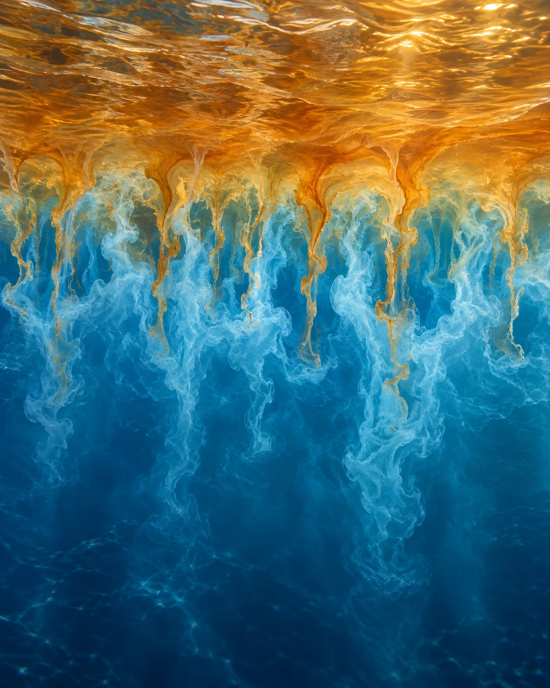
Warm-colored and cool-colored filaments interleave at an imagined water-layer boundary.
The colors distinguish conceptual water parcels and are not actual seawater colors. Filament shapes illustrate unequal exchange rather than a measured ocean flow.

Stability depends on which exchange you allow

This is the core of salt fingering, one form of double-diffusive convection. “Double” refers to two contributors to density that spread at different molecular rates. Heat diffuses much faster than salt in water, so an initially stable arrangement can develop smaller-scale motions.

A descending warm, salty parcel can lose heat and become denser than nearby water. A rising cold, fresh parcel can gain heat while retaining a relative lack of salt. Narrow interleaving motions can grow under suitable conditions. The colors in the illustration make those processes legible; ocean water does not separate into amber and blue substances.

A WHOI account of its Atlantic tracer experiment explains the large contrast between heat and salt diffusion and connects the small structures to measurable mixing. The important statement is about rates of exchange, not salt sinking independently as little solid threads.

Give a parcel a simpler ocean

The model below calculates only a parcel’s approximate density contrast. It is not a simulation of fingers. Start with a parcel 4°C warmer and 0.5 practical-salinity units saltier than the reference water. In the chosen linear approximation, that parcel is about 0.43 kilogram per cubic metre lighter.

Change a parcel’s buoyancy

Adjust temperature, salinity and heat exchange; inspect a linear density budget without pretending to calculate a mixing flux.

Open change a parcel’s buoyancy in its own window.

Now remove three quarters of its temperature excess while holding its salt contrast fixed. The example becomes about 0.18 kilogram per cubic metre denser than the reference. Nothing magical happened to the salt. The two competing contributions to density changed unequally.

These are original illustrative inputs with constant coefficients. Real seawater’s expansion and salinity effects vary with temperature and pressure, and salt also diffuses. The calculation cannot predict the growth rate, size or mixing efficiency of a real finger. It isolates one step in the mechanism so that the sign change is easy to inspect.

A staircase in a profile

Some ocean regions contain a thermohaline staircase: relatively well-mixed layers separated by sharp interfaces in temperature and salinity. Salt-finger activity can be concentrated at those interfaces. It is a structure in a vertical water profile, not a staircase on the seafloor.

The WHOI experiment near Barbados released tracer around 400 metres deep and revisited it nine months later. Its vertical spreading, considered with microstructure measurements, supported substantial mixing associated with salt fingers. The interpretation drew on several observations rather than on the visual appearance of a layered profile alone.

The original review by oceanographer Raymond Schmitt gives the wider physical framework for double diffusion. It helps distinguish salt fingering from the other common arrangement, in which colder, fresher water overlies warmer, saltier water and a different type of double-diffusive behavior may occur.

Do not make every small staircase into the same result

Observations of a daytime thermocline in the northeastern Arabian Sea examine salt-finger conditions in a much shallower and more rapidly changing setting. Such work extends the question beyond a permanent deep staircase. It does not mean that the Barbados flux estimate can be applied unchanged to the upper ocean everywhere.

Shear, ordinary turbulence, rainfall, solar heating and changing currents can alter or erase the conditions that fingers need. Recognizing a possible instability is therefore different from measuring its contribution to the local heat or salt budget.

Three checks for a double-diffusion claim
  1. Find which layer is warmer and which is saltier. A density profile by itself hides that competition.
  2. Ask whether the proposed mechanism is salt fingering or another double-diffusive arrangement.
  3. Look for a flux estimate, tracer result or microstructure evidence before translating a pattern into a mixing rate.

The fascination lies in the scale change. A water column can resist bulk overturning while permitting small parcels to exploit unequal exchanges. A seemingly stable arrangement can therefore contain an active, carefully constrained route to mixing.

Sources and further exploration

Explore all 80 new articles · Browse the complete illustrated collection

Keep exploring at Incoprea.

Thursday, October 22, 2026

Satellites Can Read the Earth in Signals They Were Never Meant to Receive

A navigation signal has an intended destination: a receiver that wants to know where it is. But radio waves are generous. Some reach the ground or sea, scatter, and continue into space. To a carefully designed satellite, that unwanted echo can become a measurement of the surface it touched.

Illustration of a navigation satellite and a receiver satellite with conceptual radio paths reflecting from ocean and floodplain.
Illustration of GNSS reflection geometry. Paths, sizes, and orbital distances are schematic; this is not a satellite image or measurement.

This is GNSS reflectometry: using reflected signals from global navigation satellite systems. Its appeal is not simply thrift. The reflections contain information that a direct signal does not, because their path includes an encounter with water, soil, vegetation, or ice.

Borrowing a transmitter changes the instrument

Ordinary radar sends out a pulse and listens for its return. A reflectometry mission can listen to transmissions already being broadcast by navigation satellites. The transmitting and receiving spacecraft are separate, and the reflection geometry changes as both move. This is a bistatic measurement rather than an echo returning to its own source.

NASA’s CYGNSS mission put this approach to work with a constellation of small spacecraft. The mission was designed to study ocean surface winds in tropical cyclones. The underlying chain is indirect: winds affect surface roughness; roughness alters how navigation signals scatter; the received pattern is interpreted with a physical model and calibration.

That chain is the article’s central caution and its main source of interest. The satellite is not feeling the wind. It is observing one consequence of the wind, amid other factors that also influence the signal. The quality of the inference depends on understanding that middle step.

A calm reflection and a rough one

Imagine a perfectly smooth mirror. For a particular arrangement of transmitter and receiver, a small region supplies a strong, organized reflection. Replace it with many tilted facets and the reflected energy spreads over a wider area and a different range of arrival delays. Ocean waves provide a constantly moving version of those facets.

The CYGNSS receiver organizes its observations into a delay-Doppler map: received power sorted by timing delay and frequency shift. NASA’s first-light explanation describes how reflected signal strength and roughness connect to the measurement. A delay-Doppler map is not a conventional photograph. Its axes describe the signal, not a simple north-up landscape.

As a reading exercise, replace the phrase “the satellite sees stronger winds” with “a retrieval estimates winds from a changed scattering pattern.” The second description sounds less immediate, but it tells you where calibration, modeling, and uncertainty enter.

Why clouds do not make this an optical camera

Navigation signals use microwave wavelengths. That makes them useful where visible-light views are obscured by cloud, and it helps the original cyclone application. It does not make the measurements immune to every atmospheric, surface, or instrument effect. Wavelength is a choice about which interactions matter, not a universal invisibility cloak.

The mission’s technical background material traces the wind-retrieval approach through modeling and earlier aircraft observations. That lineage is valuable: an elegant space concept becomes an operational measurement only after comparisons with other ways of measuring the same world.

The surprise on land

Water also changes how land reflects a microwave signal. Standing water can yield especially strong reflections, and soil wetness changes electrical properties. Researchers consequently investigated uses beyond the original ocean-wind task, including flood extent and soil moisture.

NASA’s 2018 account of flood detection describes this extension. The important word is extension: a mission designed for one geophysical target can reveal a different one when scientists examine its observations in a new context. It is not evidence that every reflection yields an equally accurate measurement of every surface property.

Vegetation, roughness, topography, and the reflection geometry complicate the land problem. A bright return does not, on its own, distinguish all combinations of wet soil, smooth inundation, and vegetation cover. Retrievals need additional information or assumptions, and their accuracy has to be evaluated for the setting in which they are used.

Build a retrieval chain on paper

Take a sheet and divide it into four boxes. Put “measured radio signal” in the first, “surface scattering” in the second, “estimated surface property” in the third, and “decision” in the last. Now try two versions:

  1. Ocean: signal pattern → roughness → estimated near-surface wind → cyclone research.
  2. Land: signal reflectivity → water-related surface response → estimated wetness or inundation → flood assessment.

Between every pair of boxes, add one assumption and one possible check. For example, the wind version needs a relationship between roughness and wind; an independent buoy observation can help test it. The land version needs to account for vegetation; field measurements can help reveal where that account fails.

This is a conceptual activity, not a recipe for processing satellite observations. Its value is that it prevents the final decision from hiding the inferential steps beneath it. Many useful environmental products are several steps removed from the raw detector reading.

One signal, more than one path to understanding

A NASA collaboration using aircraft-based receivers illustrates a further possibility: similar reflection measurements can be explored from platforms other than dedicated satellites. The transmitter infrastructure already exists; researchers can change where and how they listen.

That is the deeper idea worth carrying away. A signal can be useful twice: once for the purpose its engineers intended, and again because the world modifies it on the way. The scientific invention is the disciplined reading of that modification. The echo is not waste after all; it is a record of an encounter.

The same echo can improve when the calibration changes

A satellite dataset has a version number for a scientific reason. The recorded bits are only one stage in the route to a geophysical product. Antenna response, transmitter properties, instrument quantization, and the geometry of the reflecting area all influence how those bits become calibrated power or scattering strength.

Compare NASA’s records for CYGNSS Level 1 version 2.1 and version 3.1. The earlier release lists changes involving coordinate frames, antenna patterns, and the specular point. The later one documents revised antenna calibration and a correction to coarse quantization effects that had contributed to persistent location-dependent biases. These are descriptions of particular releases, not a recommendation to select either as the current product.

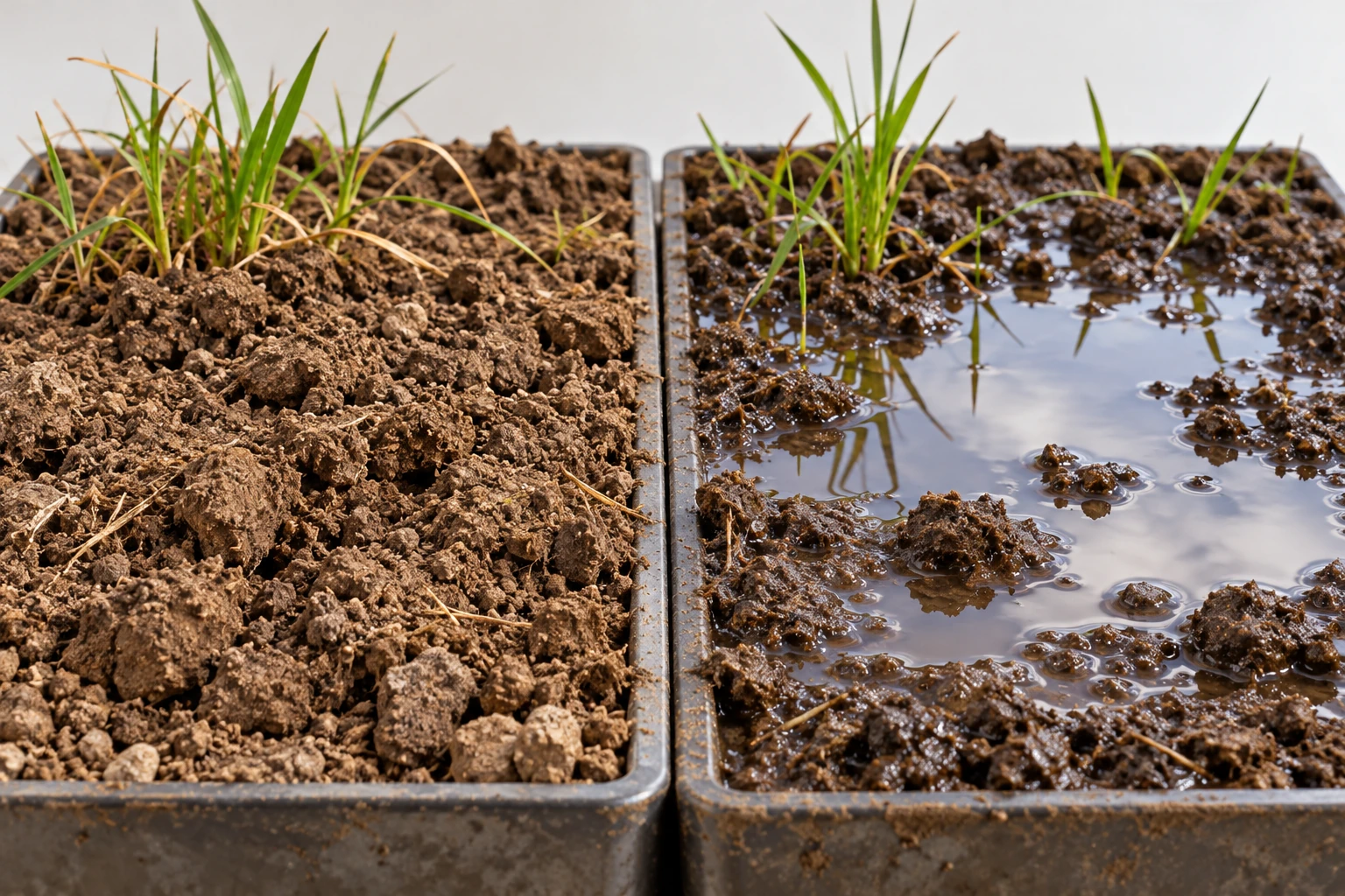
Two soil trays with comparable texture, one dry and one waterlogged
Surface comparison for thinking about wetness and roughness; it is not satellite data.

This gives a more subtle explanation for a changed map than “the ground became wetter.” The planet can change, but the processing can change too. A comparison that mixes releases without checking their definitions can place both effects in the same apparent environmental trend.

A small data detective exercise

Imagine an invented study of two fields. In the first analysis, field A has a reflectivity index of 12 and field B has 10. A recalibration changes them to 11 and 11. No new rain has fallen between these two analyses: they use the same observations. The initial contrast was sensitive to the measurement model. That does not establish that the two fields truly have identical moisture, either; the index remains an indirect observable.

Write a comparison note with five entries: observation dates, product level, release version, units, and quality screening. Then add the surface explanation you want to test. Which entries describe the Earth, and which describe the way the instrument and software represent it?

Repeat the exercise with a genuinely later observation processed using the same release. This time an environmental explanation becomes more plausible, but vegetation, roughness, and geometry still need attention. Good calibration does not eliminate the retrieval problem. It makes that problem better defined.

The photograph-like surface comparison above is deliberately not a radio measurement. It supplies two recognizable environments to think about. The numerical evidence would remain in the calibrated observations, their uncertainty, and the retrieval documentation. Keeping those roles separate lets an engaging illustration support the article without silently becoming its proof.

What a map’s blank space can mean

A constellation does not measure every location at the same instant. The navigation transmitter, receiving satellite, and surface must form a usable geometry, and individual observations then pass quality checks. A map assembled from them can therefore have gaps that reflect sampling or screening rather than a dry or calm surface.

Before using any environmental image, read the time interval, footprint size, quality flags, and legend for missing values. A daily composite can contain observations made hours apart; a colorful grid cell can summarize an area larger than a field. These are ordinary properties of remote measurements, but they matter when comparing a satellite product with an observation made at one place and one moment.

Sources and a next step

Continue exploring art, ideas, and unexpected connections at Incoprea.

Antarctica’s Hidden Lakes Can Fill, Drain, and Move the Ice Above

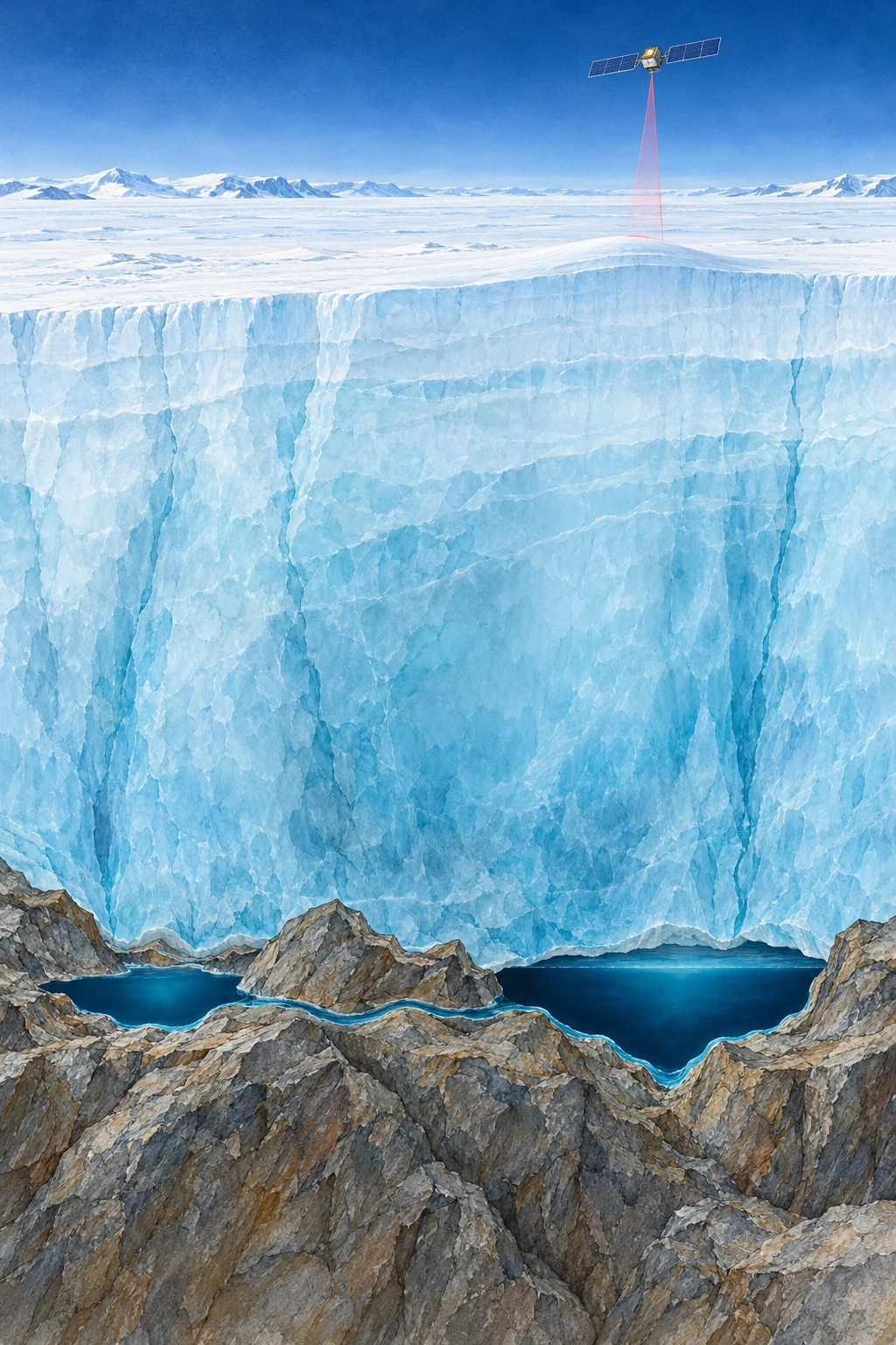
Painted cutaway of thick Antarctic ice above two liquid reservoirs connected along a rocky bed, with a satellite overhead.
Conceptual cutaway of basal lakes. Ice depth, lake shape, and satellite distance are compressed and are not observations of a named site.

Above an Antarctic lake, there may be no shoreline, no open water, and no visible basin. There may instead be a broad, almost featureless ice surface. Yet that surface can rise as water accumulates far beneath it, then sink as the hidden reservoir drains.

This is one way scientists study active subglacial lakes without drilling into every one. They measure changes in the top of the ice and work backward toward a hydraulic system at its base. The result is a continent with moving water hidden beneath an apparently frozen exterior.

Liquid water does not require a warm afternoon

At the base of an ice sheet, geothermal heat, friction, pressure, and insulation help determine whether water can remain liquid. It is misleading to picture every basal lake as surface melt that recently fell down a crack. The sources and connections vary with the glacial setting.

NASA’s early account of Antarctic subglacial lakes explains how interconnected reservoirs can fill and drain beneath fast-moving ice. Water follows hydraulic potential, which depends on pressure as well as bed elevation. A simple contour map of the bed cannot by itself tell the whole drainage story.

Imagine pressing down on a flexible water-filled bag resting on an uneven table. The water’s preferred route is influenced both by the table and by your applied pressure. This is only a conceptual analogy—the ice, sediment, and conduits are much more complicated—but it helps separate a subglacial system from an ordinary hillside stream.

The satellite measures the roof

Repeated altimetry compares the ice surface at different times. A localized rising or falling patch, with the appropriate spatial and temporal behavior, can indicate a filling or draining reservoir below. NASA’s 2021 ICESat-2 report describes improved measurements and the identification of additional active lakes.

The distinction between observation and inference matters. The laser does not pass through a kilometer of ice and bounce off the lake bottom. It measures the upper surface. Researchers must separate a basal-water signature from snowfall, ice dynamics, firn changes, and other processes that also alter that surface.

A useful figure should therefore show a time series, a footprint, and a surrounding comparison area. A single colorful depression is less informative than a repeated pattern of change supported by neighboring observations and an explanation of alternatives.

Three kinds of evidence to keep separate

What a hidden-lake claim can rest on
ObservationWhat it supportsWhat it does not show alone
Repeated localized surface uplift and subsidenceActive storage change beneath the iceA direct view of water chemistry or bed shape
Radar reflections compatible with a wet bedThe presence and geometry of a possible reservoirA complete filling-and-draining history
Direct clean-access samplingProperties of the sampled water and sedimentConditions in every other lake

These approaches can strengthen one another. Their conclusions still need to match their reach. An inventory of active lakes is not interchangeable with an inventory of every subglacial lake, because a stable reservoir may not produce a detectable surface cycle during the observation window.

The lake has a chemistry as well as a water level

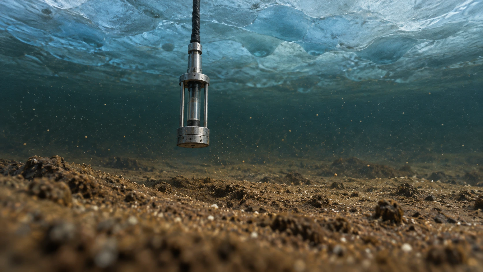
A changing ice-surface height says little about which organisms occupy the water below. For that question, the evidence chain changes from altimetry to clean access, sampling, controls, and laboratory analysis. Lake Whillans offers a particularly useful example because its water and sediments were directly sampled beneath roughly 800 meters of ice.

A small sampling instrument suspended above muddy sediment beneath an ice ceiling
Conceptual subglacial sampling scene; no organisms are depicted at visible scale.

Christner and colleagues’ 2014 study combined biological production measurements, sequencing, and geochemistry to support a microbial ecosystem with a chemosynthetic foundation. Chemical reactions can supply energy where sunlight does not arrive. That statement concerns measured processes and organisms, not an assumption that a dark lake is automatically teeming with the same community as every other lake.

The subsequent community-structure study compared lake samples with drill water and procedural controls. Its methods describe filtering potential contamination and comparing water-column and sediment assemblages. The controls are central to the discovery: finding microbial DNA somewhere in a drilling system would be much weaker evidence than distinguishing a lake-associated community from material introduced during access.

Build a three-sample evidence board

Imagine three fictional bottles: lake water, drill-system water, and an unopened procedural blank. A DNA sequence occurs in all three. What additional evidence would you need before calling it a lake inhabitant? Its presence alone does not settle the question. Relative abundance, repeated independent samples, other controls, and measurements of activity could all change the interpretation.

Now add a different sequence that is repeatedly abundant in lake sediment and rare in the controls. That pattern strengthens a lake association, but a name assigned from a short gene sequence does not establish every metabolic reaction of the organism carrying it. Direct activity measurements and chemical balances address different parts of the story.

Draw a separate arrow linking hydrology to chemistry. A filling or draining lake can exchange water and dissolved material with its surroundings, while the biology can influence what that water carries. Neither direction is captured by a single elevation map. This is why the reservoir is more than a hidden tank.

For your final note, write one conclusion supported by each instrument: laser altimeter, water sampler, and sequencing analysis. Then write one question each leaves open. The exercise gives the lake three distinct kinds of depth: its physical position, its connected water history, and the chemical life that a carefully controlled sample can reveal.

A moving inventory, with dates attached

A 2025 study by Wilson and colleagues used a decade of CryoSat-2 observations to identify 85 previously unknown active lakes. The paper’s value goes beyond adding dots to a map: repeated cycles and connected groups reveal a changing hydrological system.

ESA’s account of that study gives a total of 231 known active lakes in that inventory. That is a dated research result, not a final count for all time. “Previously unknown” also means unknown to that observational inventory, not newly created in 2025.

This is a general lesson in discovery reporting. Improved spatial coverage, a longer time series, and a better detection method can change the number of known objects without the physical population suddenly increasing by the same amount.

Try a storage calculation

Suppose a hypothetical 20-square-kilometer patch rises by an average of one meter. Multiplying area by height gives 20 million cubic meters, or 0.02 cubic kilometers, of surface-volume change. This is a scale exercise, not a claim about a particular Antarctic lake.

Turning that change into an actual water-volume estimate requires a physical model. Ice can flex beyond the reservoir outline, the measured patch may not capture the full deformation, and other elevation processes must be removed. The arithmetic is useful because it shows both how a subtle height signal can represent substantial storage and why a surface measurement is not automatically a direct volumetric gauge.

For another comparison, imagine the same surface-volume change occurring over one month and over five years. The total storage change can be equal while the implied average transfer rates differ by a factor of sixty. A lake inventory without dates would hide that difference. This is why the timing of a fill-drain cycle is as scientifically useful as its footprint: geometry describes where the reservoir is, while the sequence reveals how the system operates.

Drainage can change more than the lake

Basal water influences the conditions under which ice moves. Its routing and pressure matter, so “more water means faster ice” is not an adequate rule for every situation. Efficient channels can behave differently from distributed, pressurized water storage.

ESA’s report on a major drainage event describes links between subglacial outflow, the grounding-zone environment, and ocean melting. Such results make the hidden plumbing relevant to ice-sheet evolution, while leaving substantial work in representing it in large-scale models.

The reader’s next step is to inspect a before-and-after elevation sequence rather than only a continent-wide map. Ask which lakes filled while another drained, whether their changes were simultaneous or delayed, and what uncertainty remains about the route between them. Antarctica’s apparent stillness then becomes a measurement challenge: the most revealing movement may be a small rise in a roof whose water is out of sight.

Sources and a next step

Continue exploring art, ideas, and unexpected connections at Incoprea.

Famous Last Meals is now in paperback — stories, history and 25 recipes

Famous Last Meals: Stories, History, and Recipes is now available in paperback on Amazon. The illustrated collection brings together 23 his...