The Nocturnal Low-Level Jet: A Fast River of Air Above a Quiet Night

Conceptual illustration of a nocturnal low-level jet. Airflow streaks are visual aids, not visible air or measurements of a specific night.

The grass can be almost still while a fast stream of air moves a few hundred meters overhead. On a warm-season night in the Great Plains, the strongest low-level wind may be above the cooled surface layer rather than at your face.

The nocturnal low-level jet is important partly because of that separation. It can transport moisture and momentum through a night that feels quiet on the ground, helping shape the environment in which thunderstorms develop and persist.

Sunset changes the coupling

During daylight, turbulent mixing connects a deeper atmospheric layer with the surface. After sunset, surface cooling can produce a stable layer that reduces this vertical exchange. Winds above the most strongly cooled layer become less constrained by surface friction, and their adjustment can produce a wind-speed maximum.

The rotating Earth matters too. The wind’s adjustment includes an inertial oscillation, while regional pressure gradients, terrain slopes, and large-scale weather provide additional influences. There is no single switch that turns every low-level jet on at sunset.

The National Weather Service glossary identifies the common warm-season nocturnal southerly wind maximum over the Plains. Its training discussion also distinguishes nocturnal jets from low-level maxima associated with midlatitude cyclones. The same short label can cover mechanisms that overlap but are not identical.

Low does not mean surface

A jet is a maximum within a vertical wind profile. To establish one, observations must show how speed changes with height, including above the maximum. A strong wind reported at one level does not by itself reveal the full shape.

Picture two profiles. In the first, speed rises steadily from the ground to the top of the chart. In the second, it rises, reaches a peak, then declines. Only the second sketch demonstrates a local low-level maximum within the observed layer. The first might still contain one higher up, but the available profile has not shown it.

This is why a surface anemometer and an upper-air sounding answer different questions. Their disagreement can be a real atmospheric structure rather than a faulty instrument.

The night storms that prompted a field campaign

The 2015 PECAN campaign—Plains Elevated Convection at Night—focused on warm-season precipitation over the southern Great Plains. Its research setting included a stable boundary layer, a nocturnal low-level jet, and instability located above that stable layer.

That combination challenges the simple expectation that thunderstorms must be fed by warm air rising directly from a hot afternoon surface. Elevated inflow can supply storms after the ground layer cools. The jet helps move moisture, but storm initiation and maintenance also depend on lift, instability, boundaries, and existing storm systems.

Correlation between a stronger jet and an intense nocturnal convective system does not make jet speed a complete storm forecast. The physical setting has several ingredients, and their arrangement in space and time matters.

What the instruments add

PECAN’s instrument overview describes a combination of mobile and fixed profiling systems, radars, lidars, soundings, and aircraft. These methods were chosen to observe both the winds and the thermodynamic structure that ordinary surface observations could miss.

A wind profiler helps identify the jet’s height and evolution. Temperature and humidity profiles reveal the stable surface layer and potential elevated instability. Radar follows precipitation and storm organization. Combining them makes a causal account more testable than looking at a dramatic radar image alone.

Measurements also sample different volumes. A balloon drifts, a radar scans, and an aircraft traverses a path. A good analysis accounts for those sampling differences rather than assuming all instruments saw the same parcel at the same instant.

Try a moisture-transport thought experiment

Imagine a current of air carrying the same water-vapor concentration on two nights. If it moves twice as fast through the same cross-sectional area for the same duration, its idealized vapor transport doubles. Now imagine the faster current is much drier: the final transport need not double at all.

This is why wind alone is not the water budget. Moisture content, depth, direction, and duration belong in the account. The example deliberately leaves out convergence, condensation, and changing geometry; it illustrates one part of transport rather than predicting precipitation.

Next rotate the flow so that it runs along a storm boundary instead of crossing it. The same speed can feed a system differently. Direction and the location of the receiving weather feature are as important as the number on a wind-speed scale.

For a simple profile test, put a ten-meter-per-second wind at the surface, a twenty-meter-per-second wind above it, and a fifteen-meter-per-second wind higher still. You have drawn a maximum. Now remove the highest observation. The remaining data show increasing speed but no confirmed peak. The atmosphere has not changed; the evidence available to describe it has. This small example explains why incomplete soundings deserve a different conclusion from complete profiles.

A reading guide for a nighttime wind plot

1. Check whether height is above ground or above sea level.
2. Find the speed maximum and confirm observations extend above it.
3. Compare direction as well as speed through the profile.
4. Read temperature and humidity alongside the wind.
5. Look at several times, because the jet evolves during the night.

For a real severe-weather situation, use official forecasts and warnings. This guide is for understanding archived or educational profiles, not for making a personal flight or storm-chasing decision.

A long history of asking where the maximum is

Bonner’s 1968 low-level-jet climatology illustrates how the subject became a systematic question about frequency, geography, height, and time of day. Modern observing networks add detail, but the basic discipline remains: define the feature, sample its profile, and compare many cases.

The nocturnal jet changes how a quiet evening should be imagined. Calm at the surface is a local observation. Above it, the atmosphere can be busy transporting the ingredients of tomorrow’s rainfall.

Sources and a next step

• NWS: low-level jet glossary
• NWS training: types of low-level jets
• NCAR EOL: PECAN field campaign
• NCAR EOL: PECAN instruments
• Bonner 1968: climatology of the low-level jet

Continue exploring art, ideas, and unexpected connections at Incoprea.

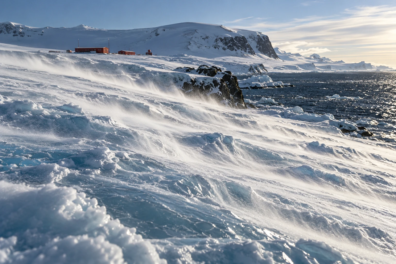
Katabatic Winds: When a Cold Ice Sheet Sends Air Downhill

Illustrative Antarctic wind scene, not a photograph or evidence of wind speed at a real station.

On an Antarctic slope, the ground can make the wind. Air near the radiatively cooled ice becomes colder and denser than air at the same level away from the slope. Gravity gives that dense layer a downhill component of motion.

This is the katabatic mechanism. Its simplicity is appealing, but the continent’s actual wind is a negotiation among buoyancy, surface drag, terrain, Earth’s rotation, and the surrounding weather. A downhill arrow is the first sketch, not the finished explanation.

A cold layer with somewhere to go

Antarctica’s ice surface rises from coastal margins toward a high interior. Cooling near that surface can generate a shallow density contrast. The downslope component of buoyancy drives flow, and terrain can collect it into preferred routes.

The Australian Antarctic Program’s explanation emphasizes how the ice-sheet shape guides persistent coastal wind directions. It also distinguishes near-surface downslope winds from the stratospheric polar vortex. One is not simply the low end of the other.

Descending air can warm through compression while still being cold relative to its surroundings. “Cold air flows down” should therefore not be interpreted as an air parcel keeping exactly the same temperature throughout its journey. The driving comparison is with the environment at the same level.

Why every coastal gale is not purely katabatic

The program’s broader weather guide explains that nearby low-pressure systems can strengthen the coastal flow. The direction can look katabatic while the large-scale pressure field provides a substantial part of the forcing.

A Coats Land study by Renfrew and Anderson deliberately examined an ordinary katabatic regime rather than only exceptional extremes. Its selection criteria separated primarily buoyancy-driven cases from winds that merely resembled them in speed and direction. That is an important methodological distinction.

If you identify a mechanism only from the outcome it often produces, you risk circular reasoning. A southerly wind on a coastal slope may be consistent with katabatic forcing, but consistency is not a full diagnosis of the force balance.

The strongest wind can be above your boots

Surface friction slows the air closest to the ice. A katabatic wind profile can therefore contain a maximum above the surface, then weaken farther aloft as the buoyancy influence decreases. Its height and depth vary with the regime.

A profiling study in Coats Land used Doppler sodar and supporting observations to investigate these vertical structures. It found distinct shapes and depths under different conditions, demonstrating why a single wind measurement cannot describe the whole layer.

The study’s specific maxima are local results, not a universal specification for Antarctica. A steep, confined coastal outlet can behave differently from a broad, modest slope. A memorable extreme-wind record says little about the ordinary profile at another station.

Try the slope-and-density sketch

Draw a slope and a thin band of cooled air resting on it. Add a downward gravity arrow. Split its effect conceptually into a component into the surface and a component along the slope. The along-slope component helps you understand why even a gentle incline can support organized flow when the cooled layer extends over a large area.

Now add three complications: surface drag, a sideways rotational deflection, and an external pressure-gradient arrow. The sketch no longer predicts a straight slide down the steepest line. That is a feature of the exercise: it shows what the one-arrow cartoon leaves out.

This is not a numerical model. A real calculation needs the density deficit, layer structure, mixing, pressure field, and boundary conditions. The paper version simply keeps the important forces from disappearing behind the familiar name.

Snow is a tracer and a measurement problem

Low streamers of loose snow can reveal surface flow, while deeper blowing snow can reduce visibility dramatically. Snow movement also complicates snowfall measurements: material passing a gauge need not all be newly falling precipitation.

When looking at a photograph, distinguish a visible snow plume from the full depth of the air current. The snow’s availability, grain properties, and lifting conditions affect what you see. Clear air above a plume is still moving, even if it carries no visible tracer.

A weather report should likewise separate sustained wind, gusts, measurement height, and averaging interval. Comparing a brief gust from one station with a long-term mean from another creates a dramatic but scientifically unhelpful contrast.

In the slope sketch, make the same height drop gradual in one panel and confined to a shorter steep section in the other. Then add a narrow outlet to only one panel. The exercise does not calculate wind speed, but it reveals three geographical questions that a regional average conceals: where the buoyancy acts, how the flow converges, and what happens after it leaves the slope.

What happens when the slope ends?

A simple cartoon sends cold air to the coast and stops. Actual flows can adjust over an ice shelf or sea, interact with regional winds, or remain organized when terrain channels them strongly. Research on near-surface ice-shelf winds compares differing behavior at the Brunt and Ross ice shelves and discusses the role of confinement and adjustment.

The lesson is geographic. The same driving principle encounters different downstream environments. The coast is not a universal off switch, and a particularly strong outlet should not stand for the whole Antarctic margin.

A better way to read the landscape

On a topographic image, trace broad ice slopes, converging valleys, and the transition to flat shelf or sea. Then compare those features with a wind rose whose station, time span, and height are known. Ask whether the favored direction follows the local fall line or is offset, and whether strong events occur under particular large-scale weather patterns.

You do not need an expedition to appreciate the result. A continental ice sheet is not merely a passive white surface beneath the atmosphere. Through cooling and terrain, it helps organize the air immediately above it—and the resulting wind gives the shape of the ice a powerful, moving expression.

Sources and a next step

• Australian Antarctic Program: downslope winds and polar vortex
• Australian Antarctic Program: Antarctic weather
• Renfrew and Anderson: ordinary Coats Land katabatic climatology
• Renfrew and Anderson: vertical wind profiles
• King: winds over an Antarctic ice shelf

Continue exploring art, ideas, and unexpected connections at Incoprea.