Showing posts with label Acoustics. Show all posts

Thursday, October 22, 2026

The SOFAR Channel: An Ocean Layer That Lets Sound Travel Far

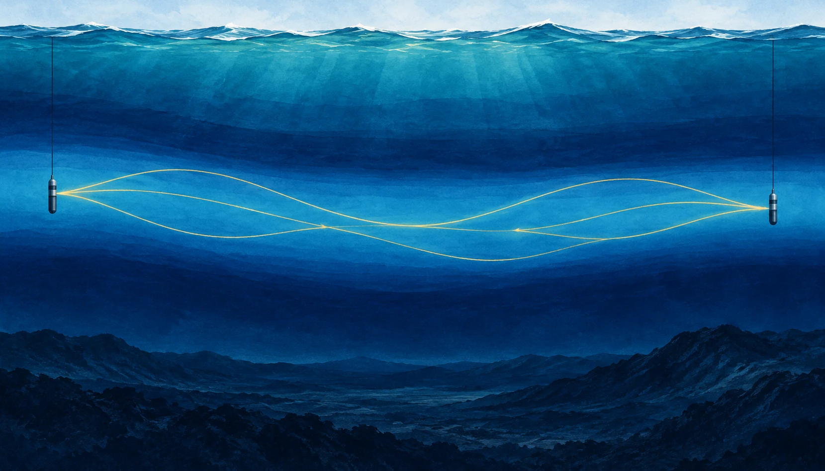
Wide ocean cutaway showing two hydrophones and gently bending gold sound paths in a blue mid-depth layer.
Conceptual illustration of a sound channel. Gold lines depict simplified ray paths, not wavelengths; scales are compressed.

A sound does not need a wall to be guided. In the open ocean, a low-frequency pulse can travel through a layer that repeatedly bends its path back toward the layer’s center. The guide is made of changing water properties. There is no pipe to find on the seabed.

The SOFAR channel—Sound Fixing and Ranging—is a reminder that the sea is not an acoustically uniform tank. Its vertical structure can matter as much as the power of the source or the sensitivity of the listener. To understand an underwater recording, you need some understanding of the water between them.

Find the slowest sound

Sound speed in seawater depends on temperature, pressure, and salinity. In a common deep-ocean profile, cooling with depth initially lowers sound speed. Farther down, increasing pressure becomes dominant and sound speed rises. Between these trends lies a minimum. NOAA’s ocean-sound explanation describes how these gradients shape the route sound takes.

Rays departing the minimum at suitable angles curve back toward it. The repeated refraction can limit losses that would occur if energy continually spread toward the surface and bottom. Low frequencies can also suffer relatively little absorption, making long-range propagation possible. The channel does not preserve every sound equally or guarantee detection at any distance.

A useful mental picture is a valley in sound speed, not a trench in the ocean floor. The axis can occur at different depths in different regions. Treat any diagram with a channel at exactly one depth as an example, not a universal ocean floor plan.

The drawing is a map of paths, not a vibrating rope

SOFAR illustrations often show a sinusoidal-looking line crossing the sea. It is easy to mistake this for the sound wave itself. Usually it represents a ray path: a simplified direction along which acoustic energy travels. The rapid pressure oscillations occur along that route; their wavelength is a separate property.

NOAA’s SOFAR guide introduces the layered-water concept. When reading the image, ask whether the horizontal and vertical scales match, whether the source sits inside the channel, and whether the drawn ray is one of several possible paths. A very flattened ocean section can make gentle bending look steep.

Those questions also explain why hearing a source does not immediately reveal its distance. A hydrophone may receive several arrivals that followed different paths. Their sequence contains information, but the loudest arrival is not necessarily the simplest geometric connection.

What made the channel important

Woods Hole Oceanographic Institution’s history and modern field account describes the long-range experiments behind the channel’s practical importance and later work on acoustic communication beneath Arctic ice. Sound can remain useful where radio and light offer limited underwater reach.

The historical experiment is best read as evidence for a physical route, not as a universal range specification. Detectability depends on frequency, source level, background noise, absorption, bathymetry, and the receiver. A successful transmission across a basin does not mean that any small speaker can communicate across the same basin.

Long-distance sound has served navigation, research, and monitoring. It also connects distant human noise sources with marine listening environments. The same physics that makes the ocean informative means a soundscape cannot always be understood by looking only at nearby traffic.

Do the travel-time arithmetic

Use a rounded sound speed of 1,500 meters per second for an idealized calculation. A 1,500-kilometer path then takes 1,000 seconds: about 16 minutes and 40 seconds. That is quick compared with a ship crossing the distance and surprisingly slow compared with an ordinary telephone conversation.

Now add a second possible path that is 15 kilometers longer. At the same rounded speed, its arrival is ten seconds later. A receiver can therefore record a sequence rather than one crisp pulse, even though both arrivals came from the same source. These are illustrative numbers, not a reconstructed ocean experiment.

The full calculation must account for how sound speed varies along each path. Temperature and currents can change the travel time too. That makes the variability both a complication for communication and a possible measurement of the water itself.

Try separating two questions in your notes: can the receiver detect the sound, and can the listener identify its source? A faint but distinctive timed signal may support a useful measurement, while a louder ambiguous sound can remain difficult to interpret. Range is only one part of a successful acoustic observation.

The Arctic does not simply copy the temperate ocean

The WHOI account describes a distinctive Arctic structure involving warm water layers of Atlantic and Pacific origin and colder intervening water. Such layering can create an acoustic duct different from the familiar deep SOFAR picture. Sea ice further changes how sound interacts with the upper boundary.

This is a useful warning against learning one attractive diagram too literally. The mechanism is refraction by a sound-speed structure; the structure must be established for the place, season, and depth of interest. A named phenomenon is a starting hypothesis about the environment, not a substitute for measuring it.

WHOI’s sound-channel animation offers another way to inspect the ray-path idea. Pause it and compare the path with the explanatory text. Ask which visible elements are actual sound recordings and which are drawn aids to understanding. The presentation combines these layers, so its caption is part of the scientific information.

A listening guide without entering the water

Use WHOI’s acoustics collection as a starting point for public recordings and explanations. Before interpreting a clip, find out whether it is raw sound, filtered sound, sped-up playback, or a sonification of non-audible measurements. A dramatic tone may be an intentional presentation choice rather than what a human diver would hear.

Then list three things you would need to infer range: the source timing or identity, a sound-speed profile, and an account of possible paths. The exercise shows how a simple recording becomes an inverse problem. The ocean has carried a message, but it has also edited the route, timing, and strength of that message on the way.

Sources and a next step

Continue exploring art, ideas, and unexpected connections at Incoprea.

Ocean Acoustic Tomography: Taking an Ocean’s Temperature With Travel Time

To take the ocean’s temperature, you can lower an instrument into it. Or you can send a sound across a large region and measure how long the journey takes. The second approach turns a route through the sea into a thermometer with an unusual shape.

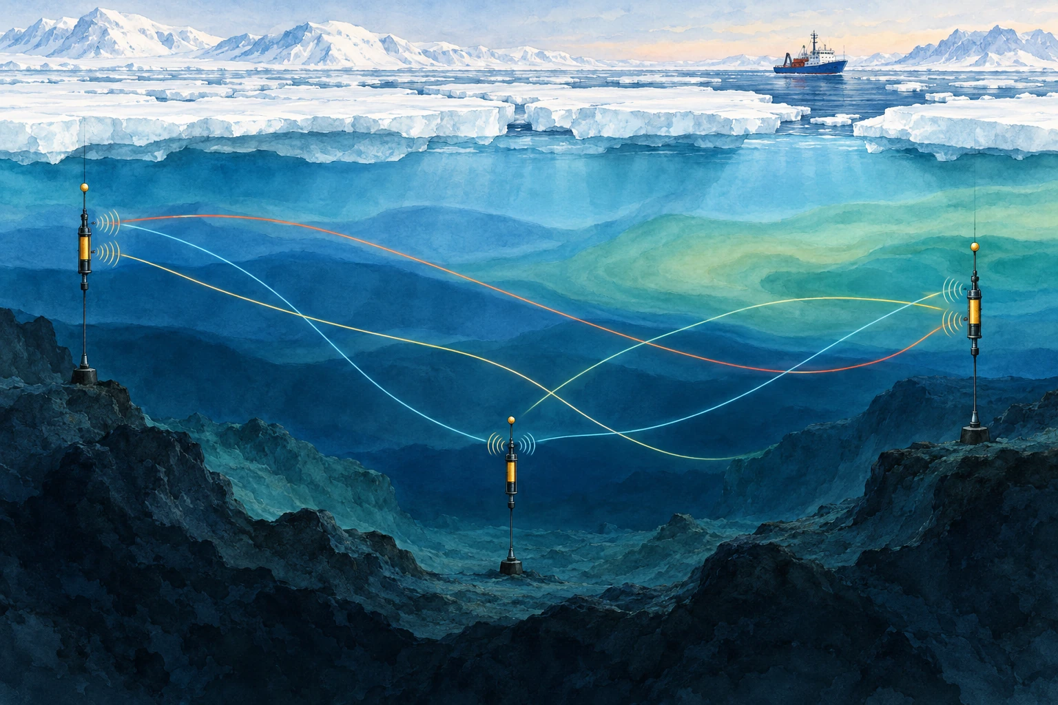
Watercolor cross section of acoustic instruments beneath sea ice, with crossing colored sound paths through different water layers.
AI-generated conceptual acoustic-tomography illustration. Colors are water-mass metaphors, not measured temperatures; paths and scales are simplified.

Ocean acoustic tomography uses travel times between known sources and receivers to infer properties of the intervening water. Its strength is also its interpretive challenge: the measurement integrates conditions along a path, rather than reporting the temperature at one point.

Time is the measurement

Sound speed depends on temperature, pressure, and salinity. In many ocean settings, temperature changes make an important contribution to travel-time variations. If the water along a known route becomes acoustically faster, a signal tends to arrive sooner, though currents and changing paths must also be considered.

WHOI’s ocean-acoustics overview describes tomography as an inverse problem: use measured travel times and known instrument locations to estimate the ocean properties responsible for them. A received pulse is not an underwater thermal photograph.

The appeal is coverage. A long acoustic path can sample a large region quickly and repeatedly. A point thermometer may be exquisitely accurate but describe only its immediate surroundings. The two approaches answer complementary questions.

The same arrival can hide different oceans

Suppose a route crosses two equal-length regions. One could warm while the other cools, leaving the overall travel-time change small. A different route that crosses only the first region could reveal the imbalance. Several crossing paths provide more information than one long connection.

This is the logic of tomography: overlapping integrals constrain a spatial pattern. The reconstruction still depends on the observing geometry, prior information, and the range of structures the available data can resolve.

Munk and Worcester’s early account of ocean acoustic tomography explains the proposal to use travel times among moorings for mapping. The method’s elegance lies in turning the ocean’s acoustic propagation from a complication into a quantitative observation.

A timing calculation

For a deliberately simple straight path of 1,000 kilometers and a uniform sound speed of 1,500 meters per second, the travel time is about 666.7 seconds. Increase that hypothetical speed to 1,501 meters per second and the time becomes about 666.2 seconds—a change of roughly 0.44 seconds.

Those round numbers are not an actual experiment or a temperature calibration. They show why precise clocks can detect a small fractional change accumulated over a long route. Converting the result to temperature requires the appropriate sound-speed relationship and an account of pressure, salinity, currents, and path geometry.

It also explains why source and receiver motion matters. A mooring that shifts changes the distance. If that shift is ignored, the analyst may assign its timing effect to the water instead. Surveying and position estimation belong inside the measurement chain.

Send sound both ways

A current can help sound travel in one direction and oppose it in the other. Reciprocal measurements—sending between two endpoints in both directions—can help distinguish a shared sound-speed contribution from an along-path flow contribution.

In an idealized uniform example, add a small current speed to the sound speed for the downstream trip and subtract it for the upstream trip. Their mean and difference then contain different information. Real analyses account for ray geometry and variable currents; the simple arithmetic is a conceptual doorway, not the full inversion.

Accurate reciprocal comparison also requires attention to timing. If the ocean changes substantially between transmissions, the paths are not sampling identical conditions. A carefully designed schedule is part of making the separation meaningful.

Why the Arctic is an especially interesting place to listen

Sea ice complicates access for ships and some satellite observations of the underlying ocean. Sound can cross beneath it. A 2026 Scripps report describes research using acoustic travel times to track Arctic ocean temperatures under the ice, providing a way to study variability in a difficult environment.

Read that capability as a complement to other measurements. Instruments that profile temperature and salinity help constrain the inversion; acoustic observations add broad path coverage and repeated sampling. An acoustic average is useful precisely because it is different from a single profile.

A reported “temperature change” should specify the depth range, region, weighting, and uncertainty. Without those details, two observing systems may appear to disagree when they actually sampled different parts of the ocean.

Paths are bent, and sometimes supplied by earthquakes

NOAA’s sound-propagation guide explains why vertical sound-speed gradients bend acoustic routes. A transmission can produce multiple arrivals associated with different paths. Correctly matching arrivals over time is therefore an essential analysis step.

Researchers have also explored using naturally generated ocean sound associated with earthquakes. Work on vertical-slice tomography with seismic waves investigates what changing travel times from repeat sources can reveal. Natural sources offer opportunities but bring their own source-location and repeatability questions.

The family resemblance is the inverse problem: establish what traveled, where, and when before assigning a change to the medium. A natural signal is not automatically simpler because no research transmitter was deployed.

A map-reading exercise

Draw three source-receiver paths across a rectangle. Mark a small warm patch crossed by only one route, then a broad patch crossed by all three. Which pattern would be easier to distinguish from the available travel times? Add two more paths and see how the answer changes.

Finally shade the regions with no crossing paths. A smooth reconstruction might still color them, but the observations constrain them less directly. That gap between a complete-looking map and uneven information is one of the most useful things to notice in any inverse image.

The ocean’s temperature is not written on the sound like a label. It is inferred from a journey, using physics, geometry, and careful comparison. The listening becomes powerful because the uncertainties are part of the account.

Sources and a next step

Continue exploring art, ideas, and unexpected connections at Incoprea.
The Elevator With Three Working Buttons

Case 50 · shortest-path challenge · Hard · About 10-15 minutes The archive elevator has a peculiar test mode. Its floor display works, but o...