Showing posts with label Atmosphere. Show all posts

Thursday, October 22, 2026

Fata Morgana: The Horizon That Builds Castles From Refracted Light

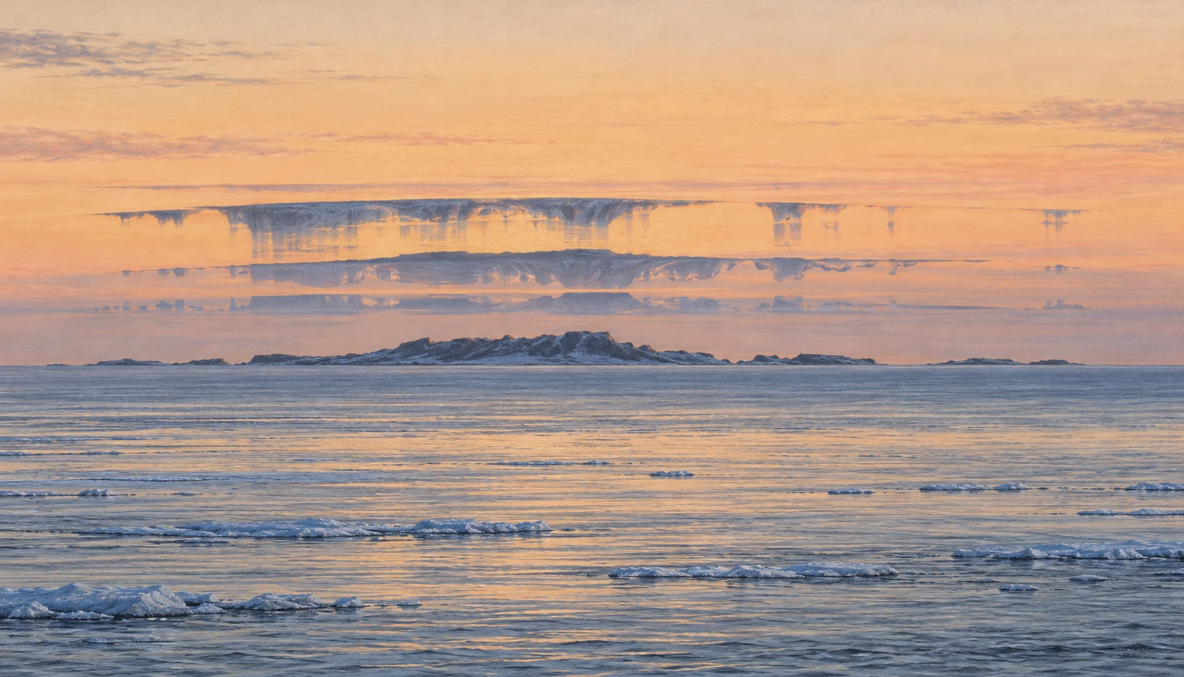
Pastel illustration of a distant cold-ocean island distorted into narrow stacked and stretched bands at the horizon.
Illustrative interpretation of a complex horizon mirage, not a documented sighting. Distortion is emphasized for visibility.

A distant shoreline can rise into a row of towers, stretch into thin pillars, split into upright and inverted pieces, then collapse back into a low strip of land. The landscape has not rebuilt itself. The route taken by its light has changed.

A complex mirage commonly called Fata Morgana can give the horizon this architectural appearance. Its fascination comes partly from a mismatch: your visual system tries to interpret familiar solid objects, while the atmosphere delivers a vertically scrambled image.

Start with an actual object

A mirage is not a hallucination. Light from real scenery reaches the observer along bent paths through air with a changing refractive index. A camera can record the resulting image. What becomes unreliable is the straightforward assumption that the object lies in the direction from which the arriving ray appears to come.

Atmospheric-optics researcher Andrew Young’s introduction at San Diego State University explains how temperature-dependent refraction creates mirages. The observer traces the final direction backward as though the ray had traveled straight. When the actual path was curved, that construction assigns the object an altered apparent position.

This makes a mirage a useful distinction between reliable detection and reliable interpretation. You truly received light. Its apparent direction does not necessarily provide the undistorted geometry you expected.

Layers can rearrange a horizon

Over a cold surface, warmer air can lie above colder, denser air. Strong vertical refractive gradients can produce superior mirages and optical ducts. Complex structures allow several ray paths to connect different parts of a distant object with the observer, producing stretching, compression, inversion, and multiple images.

Young’s detailed Fata Morgana discussion emphasizes the striking vertical elongation and apparent architecture associated with the name. It also shows why a picturesque historical description is not a complete physical diagnosis. Small changes in observer height and atmospheric structure can substantially change the display.

The mirage’s narrow vertical zone matters. Popular illustrations sometimes put a fully formed castle high in the sky. Actual complex horizon mirages tend to transform distant scenery within a compressed region near the apparent horizon. A giant fantasy city is a poor model of what an observer is looking for.

The name is less tidy than the physics

The American Meteorological Society’s glossary explicitly notes that the precise circumstances under which the term should be applied are ill-defined. That is a valuable limitation to retain. Not every photograph of a seemingly hovering ship establishes a complex Fata Morgana.

A superior mirage can elevate or invert an image without producing the elaborate stacking often associated with this name. Sometimes an indistinct or false horizon contributes to a floating appearance. A single cropped image may omit exactly the context needed to distinguish those possibilities.

Being cautious with the label does not make the phenomenon less interesting. It redirects the question from “Which exotic name wins?” to “Which refractive structure and viewing geometry could produce these observed features?” That is a question a sequence of observations can help answer.

A reflected-looking image without a reflecting surface

A mirage invites the eye to invent a mirror. An inverted strip below a distant object can look as though water reflects it; an inverted strip above can suggest a second floating object. But a refracted ray need not bounce from a sharp boundary. It can bend continuously through air whose optical properties change with height.
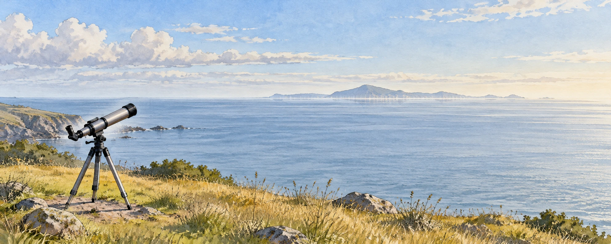
A telescope at a grassy coastal overlook facing a distant low island
Observational scene with a subtly distorted horizon; no documented sighting is implied.

Andrew Young’s ray-tracing introduction is useful here because it follows light routes rather than merely naming the resulting shapes. Its inferior-mirage example also changes the apparent horizon. The familiar “reflection” description can help identify an inverted image, but it can mislead about the mechanism.

The Atmospheric Optics superior-mirage account supplies a contrasting observational view. Instead of memorizing “hot road below, cold sea above,” compare the object, the viewer, and the refractive structure. The naming shorthand does not replace those three parts of the geometry.

A laboratory preprint on inferior mirages provides a useful contrast: controlled temperature gradients produced upright and inverted images without requiring a sheet of reflective water. That experimental analogy addresses selected optical features, not the full structure of an outdoor Fata Morgana.

Match a landmark before naming a castle

Use two views of a recognizable coast from the same general direction: one ordinary, one apparently distorted. A public example with an identified subject is preferable to an anonymous social-media crop. On tracing paper, mark only three distinctive features in the ordinary view: perhaps a notch, a mast, and a sloping headland. Search for those features in the distorted bands without forcing the intervening silhouette to match.

If the features repeat in reversed vertical order, describe that observation. If they merely stretch, describe the stretching. Leave blank any band you cannot associate with the known scene. A blank is better than a confident tower invented from a dark edge.

Now ask what a tighter crop would remove. It might hide the ordinary image below an inverted one, conceal the waterline, or eliminate a reference that shows the feature’s tiny angular height. Context can change the diagnosis even when no pixel in the surviving crop changes.

One final comparison concerns observer height. Draw two eye positions without changing the distant land. Different rays can reach them through the same layered air, so a changed image is not necessarily evidence of a changed object. The viewing position belongs in a mirage record for the same reason camera settings belong in an exposure comparison: it changes the experiment.

The aim is not to diagnose a full atmospheric profile from a scenic picture. It is to recover the real subject from a persuasive visual impression, keeping the missing information visible while the illusion remains enjoyable.

A shoreline observation notebook

If a distant coast or ship looks distorted, stay at a safe public viewpoint and make a short sequence rather than one tightly cropped photograph. Include enough surrounding water and sky to preserve the apparent horizon. Record the time, approximate viewing height, direction, and the identity of fixed landmarks when known.

  1. Take a wide contextual image before zooming in.
  2. Photograph the same feature repeatedly as the atmosphere changes.
  3. If safely possible, compare a modestly higher or lower viewpoint.
  4. Describe what changed: inversion, duplication, vertical stretch, or disappearance.
  5. Keep “possible mirage” separate from the more specific classification.

This is an observational guide, not a way to measure the full air-temperature profile from photographs alone. Nearby weather-station data may also fail to represent the thin refractive layers along a long water path.

Why height is such a strong clue

Draw a distant lighthouse and two observers at different heights. In uniform air, the geometry changes predictably as the viewpoint rises. In layered air, each observer can sample a different collection of curved ray paths. A layer that produces multiple apparent images for one viewer may place another viewer outside the necessary geometry.

The sketch is not a ray-tracing solution. It is a way to understand why “I stood beside someone and saw a different shape” need not imply imagination. The two observers may have different optical access to the same distant object.

Roland Stull’s atmospheric-optics chapter provides the broader physical framework of refraction, optical paths, and atmospheric effects. A useful next exercise is to compare its ray diagrams with an observed sequence and identify which features the simple drawing explains and which require a more complex profile.

For a useful comparison, sketch the undistorted outline of a known island from a clear-day photograph. Beside it, draw only the features you can identify in the miraged view. Leave the uncertain connections blank. Matching a recognizable notch or headland across the distorted bands is stronger evidence than deciding that the whole shape resembles a familiar building. The comparison makes interpretation answerable to a real object.

A photograph can preserve the wrong inference

Digital zoom enlarges the distorted image; it does not remove the refractive distortion. Sharpening can make a narrow bright edge look more architectural without establishing a real tower. A caption should therefore describe both the distant subject and the optical conditions inferred from the image.

There is also a scale problem. A telescope compresses a huge horizontal distance into a small frame. Without a known object, the viewer may assign an invented size to a thin band. Keeping the uncropped frame and a familiar landmark makes the picture more useful than a dramatic isolated silhouette.

The wonder survives this discipline. An ordinary island has become an experiment in how we know where things are. The apparent castle belongs neither wholly to the landscape nor wholly to the mind: it is the product of a real object, a structured atmosphere, and a particular place to stand.

Sources and a next step

Continue exploring art, ideas, and unexpected connections at Incoprea.

Kelvin–Helmholtz Clouds: When the Sky Shows Its Shear

Oil-pastel illustration of white cloud billows curling like breaking waves over a low distant ridge.
Illustration of fluctus clouds. It depicts a plausible pattern, not a recorded weather event or a turbulence forecast.

For a few minutes, a cloud edge can look like a row of breaking waves. The curls line up, topple, and dissolve. The air has briefly made a normally invisible velocity difference visible.

The familiar name is Kelvin–Helmholtz cloud. In the World Meteorological Organization’s classification, the curled supplementary feature is called fluctus. The cloud is not an ocean wave lifted into the sky. It is a tracer of an instability that fluids can share across very different settings.

Two moving layers and a disturbance that grows

Wind can change speed and direction with height. Where the shear is strong enough relative to the stabilizing effects of density structure, a small disturbance can grow into billows. The layers deform and roll, and cloud droplets or ice crystals can reveal part of the evolving flow.

The Met Office’s explanation describes the striking pattern produced when air streams move at different speeds. The key ingredient is relative motion. Two layers both moving rapidly in nearly the same way do not necessarily provide the same shear as one moving much faster than the other.

This distinction is easy to miss from the ground. A brisk surface breeze tells you about the air where you stand. It does not describe the wind profile at the cloud, which may be far above and moving differently.

A cloud feature, not one exclusive cloud species

The International Cloud Atlas defines fluctus as a relatively short-lived formation of curls or breaking-wave shapes, usually on the top of a cloud. It can occur with several cloud genera, including Cirrus, Altocumulus, Stratocumulus, Stratus, and sometimes Cumulus.

That classification is useful because it separates the cloud’s general kind from an extra feature caused by its immediate environment. A cauliflower-shaped cloud body, a layered sheet, and a thin high cloud can each acquire a transient sign of shear under appropriate conditions.

Cloud material also does not trace every moving parcel. Condensation and evaporation reveal only portions where thermodynamic conditions permit visible particles. A gap in the white pattern can therefore mean a change in visibility rather than a literal gap in the moving air.

What a still image can and cannot tell you

A clear photograph can document the curling feature. It cannot by itself provide the complete wind speed, density profile, lifetime, or strength of turbulence. Nor does every repeating ripple imply Kelvin–Helmholtz billows. Atmospheric gravity waves can create bands without the same rolled-over appearance.

A National Weather Service example of mountain-related wave clouds shows another way moving air makes repeated patterns. Comparing the two is more informative than treating all “waves in clouds” as one mechanism. In a gravity-wave sequence, oscillating air can repeatedly condense and evaporate; in shear billows, the interface itself can roll up.

Real situations can combine processes. An initial wave may create local shear or help trigger instability. A photograph can show the visible result without uniquely exposing every step that preceded it.

A five-minute observation sequence

If you notice an intriguing cloud from a safe location, take a series at a fixed framing. Include a roofline, ridge, or another stationary reference. Watch for whether the curls translate together, sharpen, merge, or fade. Record the actual interval between images; a time-lapse with unknown timing removes a useful part of the observation.

Try drawing the top edge of the same billow in three frames. The exercise distinguishes change of shape from simple movement across the sky. If only a single image survives, describe the shape you can support rather than inventing a life history for it.

Do not use this activity to make aviation or storm-safety decisions. Weather professionals combine profiles, forecasts, reports, and other observations. A beautiful cloud feature is an invitation to learn, not a replacement for that information.

A sequence can also expose an observational bias. Suppose you photograph only when a curl is most distinct. The resulting collection will suggest that billows are consistently crisp and separate. Include the less spectacular frames before and after the peak, and the instability becomes an evolving process with blurred boundaries. Those ordinary frames are often the ones that make the physics easier to understand.

Give shear an opponent

The two-arrow sketch above isolates a velocity difference. Add stable stratification and the story changes: displacing a parcel vertically can bring a restoring buoyancy force. A useful diagnostic compares the strength of that restoring tendency with the square of the vertical shear. This gradient Richardson number is commonly written Ri = N²/S², where N is buoyancy frequency and S is a velocity gradient.

Three cloud billows at different stages of curling and dispersal
A cloud-form study, not a measured instability sequence.

Research on simulated billows over terrain uses this diagnostic alongside the actual flow structure. A small Ri can identify conditions favorable to shear instability. It does not promise that every such layer will display a photographable curl.

There is an especially useful logical limit. Under the assumptions of the classical inviscid, parallel-flow linear theory, Ri greater than one quarter everywhere provides a sufficient condition for stability to small disturbances. Reversing that statement into “Ri below one quarter guarantees visible billows” changes its meaning. Parker, Caulfield, and Kerswell’s study also examines finite-amplitude structures beyond a simple linear threshold. The size and history of a disturbance can matter.

Change the competition

Use the calculator to vary hypothetical N and S. Hold N fixed and double S: the diagnostic falls by a factor of four. Hold S fixed and double N: it rises by a factor of four. The squared terms are why a modest-looking profile difference can substantially change the comparison.

A shear–stratification comparison

Explore Ri=N²/S² with hypothetical gradients; no turbulence forecast.

Open this activity in its own window.

This calculator solves no fluid equations. It has no moisture, cloud formation, diffusion, terrain, or growing vortices. Its threshold note applies to an idealized mathematical setting, not an operational turbulence forecast. There is deliberately no “safe” or “dangerous” label.

For a reading exercise, imagine two photographs with equally sharp cloud curls. One has a measured wind and temperature profile; the other has only the picture. Which permits a defensible Ri estimate? The visual resemblance does not supply the missing vertical gradients.

That is the payoff of including the opponent. Shear contains energy that disturbances may draw upon, while stable layering resists displacement. A white curl is a visible consequence of an evolving competition. The number can help organize the problem, provided its assumptions travel with it.

The sky is not the only place this happens

NASA research on Earth’s magnetopause describes Kelvin–Helmholtz waves where differently moving plasma regions meet. The fluid description has additional magnetic physics there, so a cloud analogy is not a complete model of the space environment. Still, the repeated rolling boundary is a recognizable family resemblance.

NASA’s rocket observations above Alaska provide another example of investigating mixing in atmospheric layers. The scientific interest extends beyond a photogenic silhouette: instabilities can transfer momentum and help mix regions that otherwise remain separated.

This is why the shared name is powerful. It points to a mechanism that can be investigated mathematically and observed in different media, while leaving room for each setting’s additional forces, scales, and material properties.

Try a shear comparison on paper

Draw two horizontal arrows. In the first sketch make both arrows long and equal. In the second make one long and one short. The second has the stronger speed difference even if the first has the faster average flow. Now rotate one arrow slightly: direction differences also contribute to wind shear.

The drawing leaves out density stratification and thickness, so it cannot predict whether an instability will develop. Add those missing factors as notes rather than assuming shear guarantees curls. That small act is a useful scientific habit: use a simple model for one insight, then mark the parts it does not yet explain.

A row of cloud waves is fleeting partly because the process changes the conditions that made it visible. The flow rolls, mixes, and moves on. For the observer, the lasting result is a better question to ask of a still sky: which invisible differences might the next visible edge reveal?

Sources and a next step

Continue exploring art, ideas, and unexpected connections at Incoprea.
An Atmospheric River Is a Moving Water Budget, Not a River in the Sky

An atmospheric river is easiest to misunderstand when its name is taken literally. It is not a raised channel of liquid water crossing the sky. It is an elongated region of strong water-vapor transport: moist air moving fast enough, through enough of the atmospheric column, to shift a substantial water budget.

That wording matters for anyone looking at a forecast. A bright moisture plume is not the same thing as rain already falling, and the largest instantaneous transport is not the only feature that determines the result at a particular watershed.

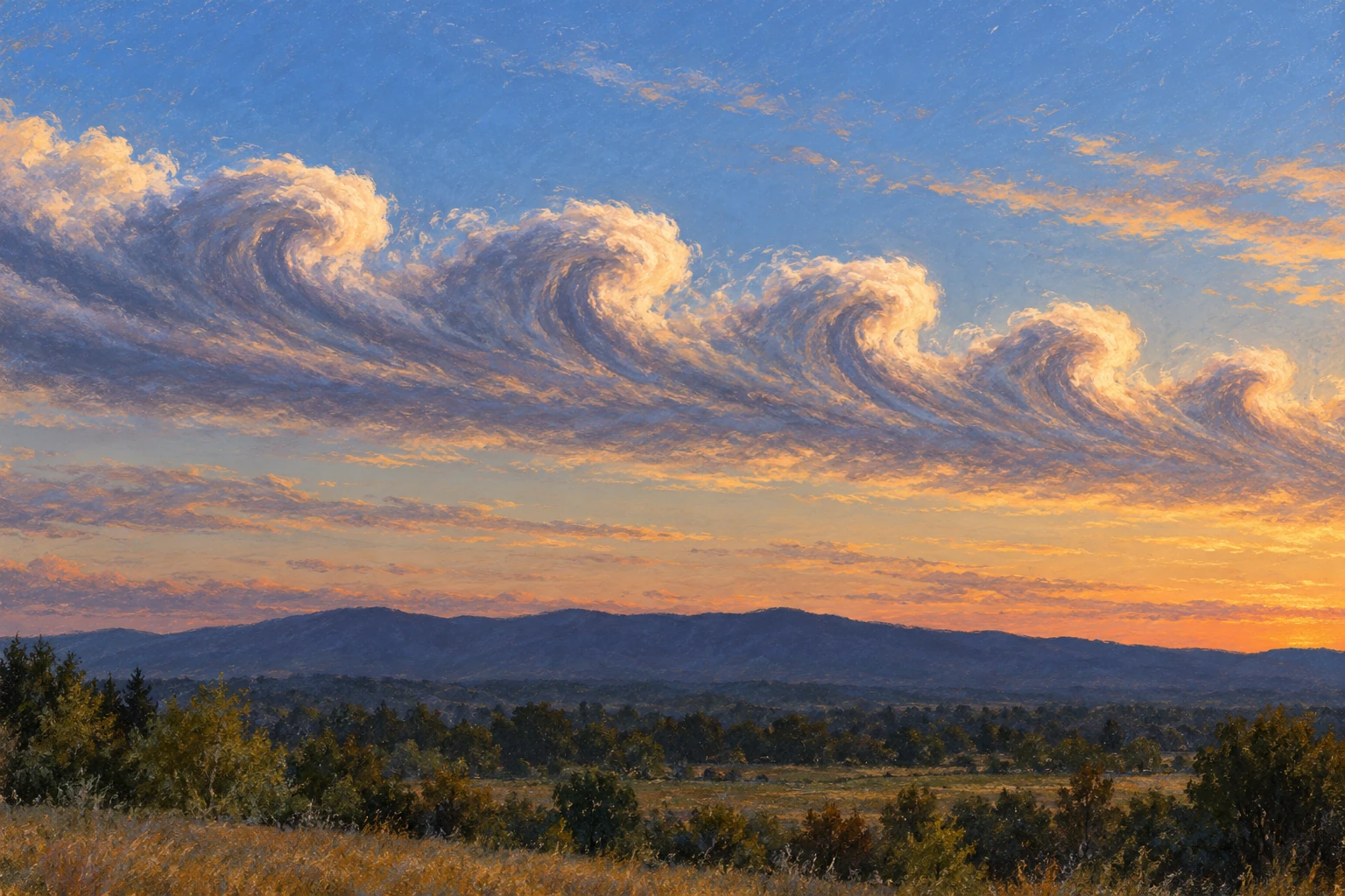
Conceptual panorama of a translucent moisture plume crossing the Pacific toward coastal mountains with rain and high-elevation snow.
Conceptual moisture-transport illustration, not a satellite observation or storm forecast. The visible plume represents invisible vapor transport.

Moisture multiplied by motion

NOAA’s introduction describes the long, narrow transport regions that play an important role in moving water vapor outside the tropics. When moist air is lifted, including over mountains, cooling can produce precipitation. The amount and location depend on the weather system and terrain.

The diagnostic quantity often shown is integrated vapor transport, or IVT. It combines water-vapor content with horizontal wind through a vertical atmospheric column. Its common unit is kilograms per meter per second: transport through a vertical curtain of unit width.

That unit is different from millimeters of rain. Turning transport into rainfall requires knowing how much moisture converges, rises, condenses, falls, and remains in or leaves the region. A large through-flow can pass over a location without all of it being deposited there.

Make the units concrete

Take a hypothetical IVT of 500 kilograms per meter per second across a 100-kilometer-wide curtain perpendicular to the flow. Multiplying by 100,000 meters gives 50 million kilograms per second. At 1,000 kilograms per cubic meter of liquid water, that is a water-equivalent volume transport of 50,000 cubic meters per second.

This is an idealized unit conversion, not a measurement of a named storm and not the flow of a sky-borne liquid river. It says how much water vapor crosses the selected curtain in the example. The curtain’s orientation matters: transport oblique to it needs the perpendicular component.

Now hold the transport steady for 12 hours, then imagine the same value lasting 48 hours. Four times the time means four times the cumulative transport across that curtain. Even before adding land conditions, duration changes the scale of the event.

A scale that includes time

The 2019 atmospheric-river scale developed by Ralph and colleagues combines peak IVT with duration at a location. Its categories are intended to communicate a spectrum from beneficial to increasingly hazardous conditions rather than treating every atmospheric river as a disaster.

Scripps’ explanation of the scale describes the role of the 24-to 48-hour duration range and the adjustments for shorter or longer events. A scale category is still not a complete flood forecast. It describes a transport event, while the watershed has its own recent history and vulnerabilities.

A dry catchment and a saturated one can respond differently to similar precipitation. Snow level can shift the balance between immediate runoff and stored snow. Recently burned terrain, steep slopes, drainage capacity, and reservoir operations can also change local outcomes.

Read the plume, then read the spread

CW 3 E’s forecast guide explains its plume diagrams and ensemble products. Thin lines represent different model members, helping expose uncertainty in timing, strength, and duration. A single thick forecast line is easier to look at, but can conceal a meaningful spread among plausible evolutions.

Use a forecast as a set of questions. When does transport begin? How long does it stay elevated? Do model members agree on the peak? Does the plume aim at the same stretch of coast in successive forecasts? A small landfall shift can place strong flow against a different mountain barrier or watershed.

The page also notes that its analysis representation of IVT is modeled rather than a direct continuous measurement everywhere. That distinction should travel with a screenshot. A colored map can be an analysis, a forecast, or a composite; the label determines how it should be read.

A watershed comparison

Same transport label, different setting
SettingAdditional question
Dry basin after a long rain-free periodHow much storage is available in soils and reservoirs?
Already wet basinHow quickly will new rainfall become runoff?
Mountain catchmentWhere is the snow level and how does terrain face the flow?
Recently burned slopeWhat local debris-flow guidance has been issued?

The table is an interpretation aid, not site-specific hazard advice. For an actual event, local weather and emergency guidance supply the necessary place-based information.

Here is a second scale check: if a hypothetical ten millimeters of rain falls uniformly over a hundred square kilometers, the water volume is one million cubic meters. The amount reaching a channel immediately can be much smaller or arrive later, depending on storage and routing. Comparing this rainfall-volume calculation with the earlier transport calculation shows why they are different budgets. One crosses an atmospheric curtain; the other is deposited over a land area. Keeping their units visible prevents an impressive vapor-flow number from being mistaken for an inevitable flood volume.

Why researchers fly into the uncertainty

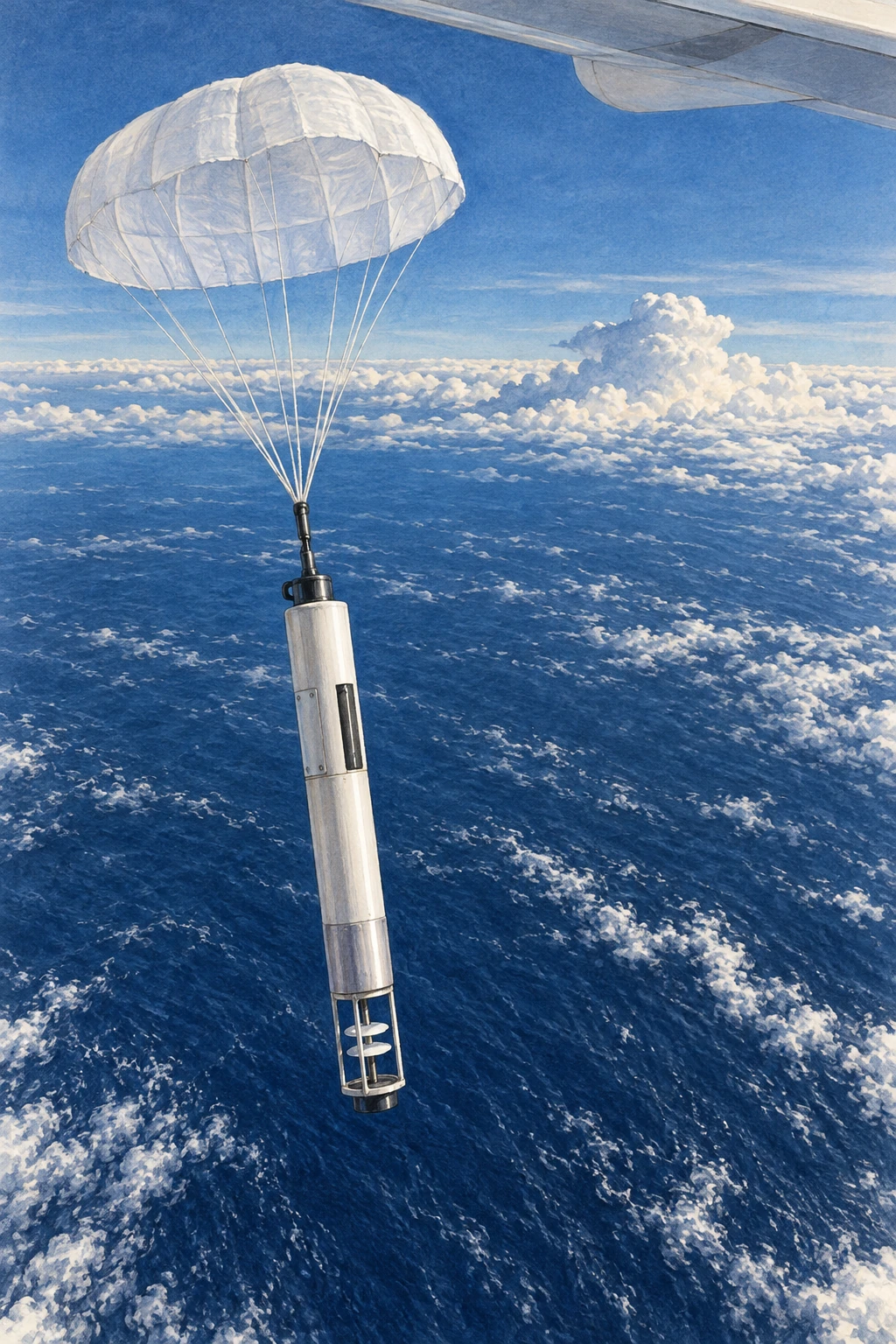
Atmospheric River Reconnaissance targets observations over the otherwise sparsely sampled ocean. Aircraft dropsondes measure vertical profiles; added observations can improve the starting state of forecast models and help researchers investigate which regions most affect later predictions.

The point is more subtle than “more data is always better.” Measurements must be placed, timed, quality-controlled, and assimilated so that they reduce the uncertainties relevant to the forecast. Sensitivity analysis helps identify where an observation can be especially informative.

After reading an event summary, try making a two-line account: one line for the atmosphere’s transport and one for the land’s response. Add the uncertainty to each. This keeps a useful scientific term from becoming a dramatic synonym for rain, and helps you see why the same atmospheric process can replenish a region’s water supply in one episode and overwhelm it in another.

How would you know the flight helped?

A research aircraft can bring back a beautiful profile and still leave a harder question unanswered: did those measurements improve the forecast people ultimately used? Testing that requires a comparison. Researchers can run a forecasting system with a selected observation set and run a matched experiment withholding those observations.

A parachute-supported research dropsonde descending over the Pacific
Illustrative research dropsonde; it is not a record of a particular flight.

A study of the 2020 AR observing campaign compared a control including reconnaissance dropsondes with a denial experiment excluding them in a specified global forecasting system. That design asks about the contribution of those data within that system and period. It does not show that aircraft are the only useful observations or that every individual flight must improve every local prediction.

A later sampling-strategy study summarized by its CW3E authors explored mission frequency and sonde spacing during a six-day 2021 sequence. Reducing temporal or spatial sampling degraded skill in the experiments reported there. The placement and repetition of observations were part of the result, not interchangeable details of flight logistics.

Design a fair forecast comparison

Use a fictional example with two forecast runs for the same storm. Run A places a heavy-rain band 100 kilometers too far north. Run B puts it 20 kilometers too far north but predicts an excessive peak amount. Which is better? You cannot answer fully until you state what is being scored.

Make three rows: location of the band, total rainfall over the watershed, and maximum point rainfall. Give each a separate assessment. A model can improve on one metric while worsening on another. One screenshot with a convincing storm shape cannot settle all three.

Next require the runs to use the same model version, forecast start time, and verification observations. Otherwise an apparent benefit might come from a different upgrade or a more favorable comparison window. Finally compare several lead times rather than selecting the one with the largest improvement.

The exercise explains why field campaigns and forecast evaluation belong together. Measuring the atmosphere improves the starting evidence. Demonstrating a useful forecast benefit needs a second experiment that follows those measurements through assimilation, prediction, and verification. The dropsonde’s descent is only the beginning of its scientific journey.

Sources and a next step

Continue exploring art, ideas, and unexpected connections at Incoprea.
The Quasi-Biennial Oscillation: A Wind Reversal Above the Tropics

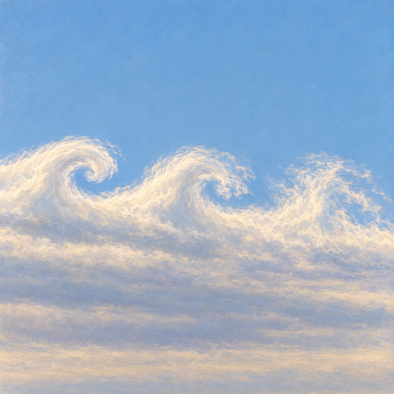
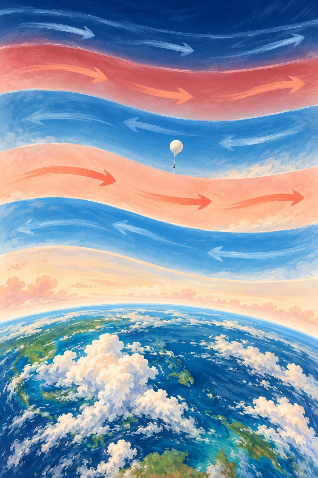
Conceptual portrait of Earth’s equatorial atmosphere with alternating blue and coral flow bands and a small weather balloon.
Conceptual illustration of alternating stratospheric wind regimes, not a measured QBO chart; heights and band thicknesses are schematic.

High above the tropical clouds, the wind can blow eastward at one height and westward at another. Over time, those broad wind regimes descend. A location that once had one direction acquires the other, then eventually returns.

The pattern is the quasi-biennial oscillation, usually shortened to QBO. Its name promises something close to two years, but its average full cycle is nearer 28 months. It is regular enough to help seasonal prediction and irregular enough to remind researchers that an atmospheric clock is not a mechanical clock.

A direction change that moves downward

The QBO concerns zonal winds—winds around the equatorial belt—in the stratosphere. NASA’s QBO data guide describes a downward-propagating wind variation, drawing on radiosondes, satellite observations, and assimilated datasets.

Downward propagation does not mean that an entire layer of air simply falls from the upper stratosphere to the lower stratosphere. It means that the phase boundaries and wind regimes appear at progressively lower heights. That distinction between a moving pattern and moving material recurs throughout wave science.

Imagine colored bands on a display that change one row at a time. A blue-to-red transition can travel downward even if no pixel moves. The analogy omits the fluid dynamics, but it prevents a misleading picture of a giant descending air conveyor.

The engine is in the waves

Waves generated in and below the tropical atmosphere carry momentum upward. As they interact with the background wind, different parts of the wave field deposit momentum at different levels. The evolving wind then changes which waves can continue upward. This feedback helps create alternating regimes.

Research evaluating QBO wave forcing in ERA 5 examines the contributions of different wave types. It is a richer problem than simply saying that equatorial heating reverses the wind on a schedule. The wave spectrum, background circulation, damping, and model representation all matter.

A numerical model also cannot explicitly resolve every relevant wave. Parameterizations represent some smaller-scale effects, and choices about them can influence whether the simulated QBO has the appropriate period, amplitude, and downward reach.

Read the striped chart as a story

A common QBO figure has time across the horizontal axis, pressure or height vertically, and color showing zonal wind. Trace a sloping edge downward and to the right: it shows a regime appearing at lower levels as time advances. At one date, different heights can have different phases.

Before naming the phase, specify the level. “The QBO is easterly” is incomplete if the speaker does not identify the pressure level or index used. A layer above may already have changed direction while the level used in a seasonal forecast has not.

  1. Read whether the vertical axis is height or pressure; pressure usually decreases upward.
  2. Check the sign convention for eastward and westward winds.
  3. Follow one level across time, then follow one regime downward.
  4. Keep measured station winds separate from a model reanalysis or forecast.

This is a reading exercise, not an invitation to infer tomorrow’s local weather from one stripe. The QBO is a large-scale influence with statistical connections, not a daily forecast for a particular street.

What happened when the clock stumbled

NASA’s 2016 account described an unprecedented disruption in the then-observed record: an unexpected wind structure interrupted the usual descent. The report posed questions about possible causes rather than declaring one proven explanation.

That date matters. A news article written while an event was under investigation is evidence of what was known then, not a final statement that no later analysis exists. It is also not evidence that the oscillation permanently stopped.

Research on the disrupted pattern’s recovery found that recovery involved a substantial phase delay. The lesson is more interesting than “the clock broke”: atmospheric regularity emerges from interacting processes and can be reorganized when unusual forcing enters the system.

Another way to inspect the chart is to compare a calendar expectation with a phase expectation. Mark a date exactly two years after one wind reversal, then find where the next comparable reversal actually occurred. The mismatch is not automatically an error in the data: the name describes an approximate rhythm. Next mark the same phase at another pressure level. You now have two kinds of difference, variable cycle length and vertical phase lag. Keeping them separate makes it easier to understand why a forecast index must state both its level and its date. A familiar label can otherwise conceal a changed definition from one discussion to the next.

The second disruption changed the question

The 2016 event was unprecedented in the observational account discussed above. It did not remain the only interruption. In 2019/20 another unusual easterly structure developed within a descending westerly regime. That later event makes a more interesting question possible: which parts of the two disruptions were alike, and which depended on a different sequence of wave forcing?

A radiosonde suspended well below a rising weather balloon over a tropical launch area
Illustrative balloon sounding; the wind regime is inferred from measurements, not visible bands.

Kang and Chun’s 2021 analysis used reanalysis to separate wave contributions during the 2019/20 event. Their account distinguishes an earlier role for Rossby-wave forcing from a later strong contribution by mixed Rossby–gravity waves. Those names describe diagnosed dynamical components; they are not objects visible in an ordinary balloon photograph.

Anstey and colleagues’ analysis compared the interruptions and examined their implications for predictability. The oscillation resumed with its phase shifted from an uninterrupted expectation. Their inference about potentially more frequent future disruptions used model projections, so it belongs in the category of research-based expectation rather than an already observed future.

Make the phase error visible

Draw a row of twelve equally spaced marks as an invented expected sequence of wind reversals. Copy it below, but delay the seventh mark and all later marks by one interval. The lower sequence has not stopped forever. It has lost the timing relationship that a forecast based on the upper sequence would assume.

Now draw a third sequence with one extra brief reversal between the sixth and seventh marks. That is a different interruption. Merely labeling both “a disrupted clock” conceals their different structures. An actual QBO analysis needs the full time–height wind pattern and momentum budget to distinguish such possibilities.

Return to a published 2019/20 figure and identify three dates: an early departure from the expected wind, the development of the anomalous easterly layer, and the later recovery. Do not assign the first to the moment of the second just because the headline names one month.

This comparison improves a common discovery story. An unprecedented observation establishes that something can happen. A second well-studied case begins to expose which mechanisms may recur and how much a useful prediction depends on them. The atmosphere’s rhythm remains useful, but its exceptions now have a history worth comparing.

How a tropical wind can matter far away

The QBO affects the stratospheric circulation and can influence conditions at higher latitudes. The Met Office’s climate-driver guide discusses its relationship with the polar vortex and winter weather probabilities, while stressing interactions with other drivers.

A changed probability is not a guarantee. ENSO, the state of the ocean and land, internal weather variability, and other stratospheric conditions can combine differently in different years. A phase can be associated with an increased chance of a type of winter without producing that winter every time.

This is an excellent place to practice probabilistic language. “Favors,” “raises the chance,” and “contributes information” are more faithful than “causes this winter” when the evidence concerns a distribution of possible outcomes.

Make a two-level timeline

Use a public QBO chart and choose two clearly marked pressure levels. Mark the dates each changes sign. Measure the lag between them, then compare a later cycle. You should expect a pattern rather than a perfectly fixed interval. Note any data gaps and avoid reading the color boundary more precisely than the plotting resolution allows.

The activity converts an abstract oscillation into something you can follow. It also shows why a single index compresses a three-dimensional evolving atmosphere. The tropical stratosphere carries an unusually recognizable rhythm, but the rhythm is made by the atmosphere each time it plays.

Sources and a next step

Continue exploring art, ideas, and unexpected connections at Incoprea.
The Nocturnal Low-Level Jet: A Fast River of Air Above a Quiet Night

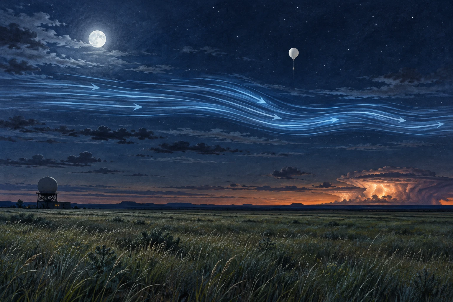
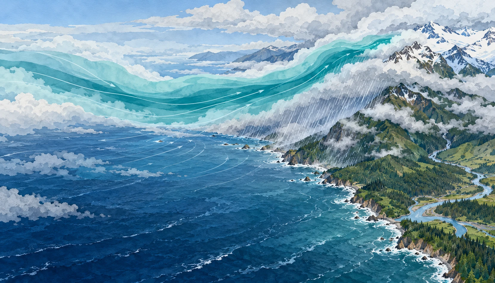
Moonlit Plains landscape with a conceptual blue airflow band above quiet grass, a weather balloon, and distant storm.
Conceptual illustration of a nocturnal low-level jet. Airflow streaks are visual aids, not visible air or measurements of a specific night.

The grass can be almost still while a fast stream of air moves a few hundred meters overhead. On a warm-season night in the Great Plains, the strongest low-level wind may be above the cooled surface layer rather than at your face.

The nocturnal low-level jet is important partly because of that separation. It can transport moisture and momentum through a night that feels quiet on the ground, helping shape the environment in which thunderstorms develop and persist.

Sunset changes the coupling

During daylight, turbulent mixing connects a deeper atmospheric layer with the surface. After sunset, surface cooling can produce a stable layer that reduces this vertical exchange. Winds above the most strongly cooled layer become less constrained by surface friction, and their adjustment can produce a wind-speed maximum.

The rotating Earth matters too. The wind’s adjustment includes an inertial oscillation, while regional pressure gradients, terrain slopes, and large-scale weather provide additional influences. There is no single switch that turns every low-level jet on at sunset.

The National Weather Service glossary identifies the common warm-season nocturnal southerly wind maximum over the Plains. Its training discussion also distinguishes nocturnal jets from low-level maxima associated with midlatitude cyclones. The same short label can cover mechanisms that overlap but are not identical.

Low does not mean surface

A jet is a maximum within a vertical wind profile. To establish one, observations must show how speed changes with height, including above the maximum. A strong wind reported at one level does not by itself reveal the full shape.

Picture two profiles. In the first, speed rises steadily from the ground to the top of the chart. In the second, it rises, reaches a peak, then declines. Only the second sketch demonstrates a local low-level maximum within the observed layer. The first might still contain one higher up, but the available profile has not shown it.

This is why a surface anemometer and an upper-air sounding answer different questions. Their disagreement can be a real atmospheric structure rather than a faulty instrument.

The night storms that prompted a field campaign

The 2015 PECAN campaign—Plains Elevated Convection at Night—focused on warm-season precipitation over the southern Great Plains. Its research setting included a stable boundary layer, a nocturnal low-level jet, and instability located above that stable layer.

That combination challenges the simple expectation that thunderstorms must be fed by warm air rising directly from a hot afternoon surface. Elevated inflow can supply storms after the ground layer cools. The jet helps move moisture, but storm initiation and maintenance also depend on lift, instability, boundaries, and existing storm systems.

Correlation between a stronger jet and an intense nocturnal convective system does not make jet speed a complete storm forecast. The physical setting has several ingredients, and their arrangement in space and time matters.

What the instruments add

PECAN’s instrument overview describes a combination of mobile and fixed profiling systems, radars, lidars, soundings, and aircraft. These methods were chosen to observe both the winds and the thermodynamic structure that ordinary surface observations could miss.

A wind profiler helps identify the jet’s height and evolution. Temperature and humidity profiles reveal the stable surface layer and potential elevated instability. Radar follows precipitation and storm organization. Combining them makes a causal account more testable than looking at a dramatic radar image alone.

Measurements also sample different volumes. A balloon drifts, a radar scans, and an aircraft traverses a path. A good analysis accounts for those sampling differences rather than assuming all instruments saw the same parcel at the same instant.

Try a moisture-transport thought experiment

Imagine a current of air carrying the same water-vapor concentration on two nights. If it moves twice as fast through the same cross-sectional area for the same duration, its idealized vapor transport doubles. Now imagine the faster current is much drier: the final transport need not double at all.

This is why wind alone is not the water budget. Moisture content, depth, direction, and duration belong in the account. The example deliberately leaves out convergence, condensation, and changing geometry; it illustrates one part of transport rather than predicting precipitation.

Next rotate the flow so that it runs along a storm boundary instead of crossing it. The same speed can feed a system differently. Direction and the location of the receiving weather feature are as important as the number on a wind-speed scale.

For a simple profile test, put a ten-meter-per-second wind at the surface, a twenty-meter-per-second wind above it, and a fifteen-meter-per-second wind higher still. You have drawn a maximum. Now remove the highest observation. The remaining data show increasing speed but no confirmed peak. The atmosphere has not changed; the evidence available to describe it has. This small example explains why incomplete soundings deserve a different conclusion from complete profiles.

A reading guide for a nighttime wind plot

  1. Check whether height is above ground or above sea level.
  2. Find the speed maximum and confirm observations extend above it.
  3. Compare direction as well as speed through the profile.
  4. Read temperature and humidity alongside the wind.
  5. Look at several times, because the jet evolves during the night.

For a real severe-weather situation, use official forecasts and warnings. This guide is for understanding archived or educational profiles, not for making a personal flight or storm-chasing decision.

A storm can send a wave ahead of itself

The jet is one part of a nighttime setting that can also support traveling disturbances. A thunderstorm’s outflow can encounter a stable lower layer and generate an atmospheric bore: a propagating adjustment of the layered air that may be followed by waves. The resulting lift can matter even where rain has not yet arrived.

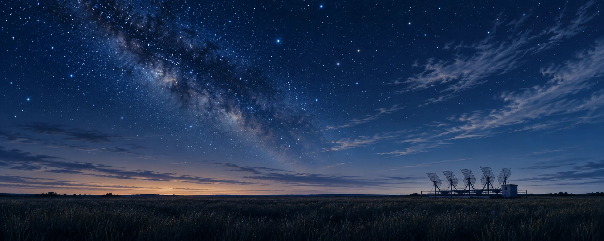
A research wind profiler beside dark Great Plains grass under a broad night sky
Quiet-ground observational scene; the instrument’s returns would reveal the air aloft.

The PECAN research overview included storm-generated wave-like disturbances among its objectives. The team’s operations plan treated bores as a specific observational target. The distinction matters: a nocturnal wind maximum and a moving bore are different features that can interact within the same environment.

Think of a layered atmosphere as having a structure that can be displaced, rather than a uniform block merely pushed across the ground. A bore can move a change through that structure while individual air parcels follow more complicated paths. The familiar wave-versus-material distinction reappears, now with implications for where elevated air may be lifted.

Three instruments, three arrival times

Imagine a fictional research site. At midnight a pressure sensor records a small step. Several minutes later a profiling instrument shows the stable layer displaced upward. Rain begins half an hour after that. These observations could motivate a bore hypothesis, but the sequence alone does not prove it. Other boundaries and local effects can alter pressure and profiles.

On paper, place the site between two additional observing stations. What would a propagating feature predict? You would expect a spatially ordered timing pattern rather than three unrelated local changes. Add a radar cross section or repeated thermodynamic profiles and specify what additional structure would strengthen the explanation.

Now move only the rain-start time. The disturbance’s apparent speed should be estimated from the observations tracking the disturbance, not from a later precipitation edge that may have a different motion. This is a small but consequential choice about what feature is actually being followed.

The activity is an interpretation of invented evidence, not a storm warning procedure. Its value is to make a quiet night less deceptively simple. A surface can cool, a jet can transport air above it, and a traveling adjustment can change the lift supplied to that air. The scientific account becomes stronger when those roles are measured separately before they are combined.

A long history of asking where the maximum is

Bonner’s 1968 low-level-jet climatology illustrates how the subject became a systematic question about frequency, geography, height, and time of day. Modern observing networks add detail, but the basic discipline remains: define the feature, sample its profile, and compare many cases.

The nocturnal jet changes how a quiet evening should be imagined. Calm at the surface is a local observation. Above it, the atmosphere can be busy transporting the ingredients of tomorrow’s rainfall.

Sources and a next step

Continue exploring art, ideas, and unexpected connections at Incoprea.
Katabatic Winds: When a Cold Ice Sheet Sends Air Downhill

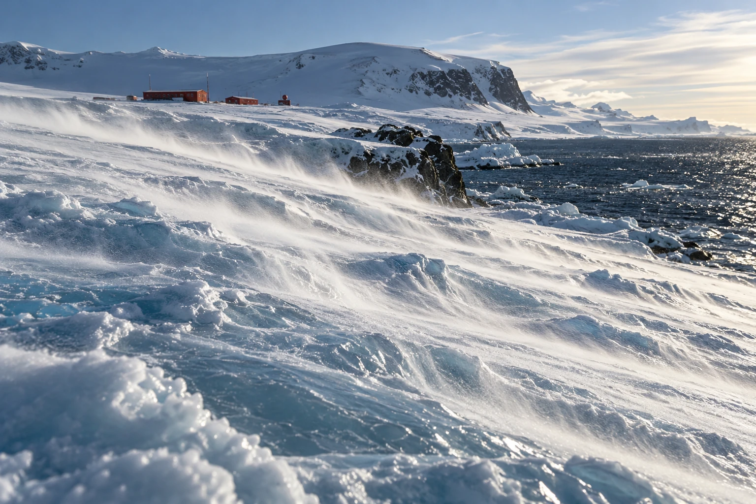
Documentary-style painting of low snow streamers sweeping down an Antarctic ice slope toward dark coastal water.
Illustrative Antarctic wind scene, not a photograph or evidence of wind speed at a real station.

On an Antarctic slope, the ground can make the wind. Air near the radiatively cooled ice becomes colder and denser than air at the same level away from the slope. Gravity gives that dense layer a downhill component of motion.

This is the katabatic mechanism. Its simplicity is appealing, but the continent’s actual wind is a negotiation among buoyancy, surface drag, terrain, Earth’s rotation, and the surrounding weather. A downhill arrow is the first sketch, not the finished explanation.

A cold layer with somewhere to go

Antarctica’s ice surface rises from coastal margins toward a high interior. Cooling near that surface can generate a shallow density contrast. The downslope component of buoyancy drives flow, and terrain can collect it into preferred routes.

The Australian Antarctic Program’s explanation emphasizes how the ice-sheet shape guides persistent coastal wind directions. It also distinguishes near-surface downslope winds from the stratospheric polar vortex. One is not simply the low end of the other.

Descending air can warm through compression while still being cold relative to its surroundings. “Cold air flows down” should therefore not be interpreted as an air parcel keeping exactly the same temperature throughout its journey. The driving comparison is with the environment at the same level.

Why every coastal gale is not purely katabatic

The program’s broader weather guide explains that nearby low-pressure systems can strengthen the coastal flow. The direction can look katabatic while the large-scale pressure field provides a substantial part of the forcing.

A Coats Land study by Renfrew and Anderson deliberately examined an ordinary katabatic regime rather than only exceptional extremes. Its selection criteria separated primarily buoyancy-driven cases from winds that merely resembled them in speed and direction. That is an important methodological distinction.

If you identify a mechanism only from the outcome it often produces, you risk circular reasoning. A southerly wind on a coastal slope may be consistent with katabatic forcing, but consistency is not a full diagnosis of the force balance.

The strongest wind can be above your boots

Surface friction slows the air closest to the ice. A katabatic wind profile can therefore contain a maximum above the surface, then weaken farther aloft as the buoyancy influence decreases. Its height and depth vary with the regime.

A profiling study in Coats Land used Doppler sodar and supporting observations to investigate these vertical structures. It found distinct shapes and depths under different conditions, demonstrating why a single wind measurement cannot describe the whole layer.

The study’s specific maxima are local results, not a universal specification for Antarctica. A steep, confined coastal outlet can behave differently from a broad, modest slope. A memorable extreme-wind record says little about the ordinary profile at another station.

Try the slope-and-density sketch

Draw a slope and a thin band of cooled air resting on it. Add a downward gravity arrow. Split its effect conceptually into a component into the surface and a component along the slope. The along-slope component helps you understand why even a gentle incline can support organized flow when the cooled layer extends over a large area.

Now add three complications: surface drag, a sideways rotational deflection, and an external pressure-gradient arrow. The sketch no longer predicts a straight slide down the steepest line. That is a feature of the exercise: it shows what the one-arrow cartoon leaves out.

This is not a numerical model. A real calculation needs the density deficit, layer structure, mixing, pressure field, and boundary conditions. The paper version simply keeps the important forces from disappearing behind the familiar name.

Snow is a tracer and a measurement problem

Low streamers of loose snow can reveal surface flow, while deeper blowing snow can reduce visibility dramatically. Snow movement also complicates snowfall measurements: material passing a gauge need not all be newly falling precipitation.

When looking at a photograph, distinguish a visible snow plume from the full depth of the air current. The snow’s availability, grain properties, and lifting conditions affect what you see. Clear air above a plume is still moving, even if it carries no visible tracer.

A weather report should likewise separate sustained wind, gusts, measurement height, and averaging interval. Comparing a brief gust from one station with a long-term mean from another creates a dramatic but scientifically unhelpful contrast.

In the slope sketch, make the same height drop gradual in one panel and confined to a shorter steep section in the other. Then add a narrow outlet to only one panel. The exercise does not calculate wind speed, but it reveals three geographical questions that a regional average conceals: where the buoyancy acts, how the flow converges, and what happens after it leaves the slope.

What happens when the slope ends?

A simple cartoon sends cold air to the coast and stops. Actual flows can adjust over an ice shelf or sea, interact with regional winds, or remain organized when terrain channels them strongly. Research on near-surface ice-shelf winds compares differing behavior at the Brunt and Ross ice shelves and discusses the role of confinement and adjustment.

The lesson is geographic. The same driving principle encounters different downstream environments. The coast is not a universal off switch, and a particularly strong outlet should not stand for the whole Antarctic margin.

The wind can help keep an ice-making opening open

At a coast, a persistent offshore wind can move newly formed sea ice away from the shoreline. The exposed or thinly covered water loses heat rapidly to cold air, allowing more ice to form. An opening can therefore be associated with active ice production rather than simply with warmth that prevents freezing.

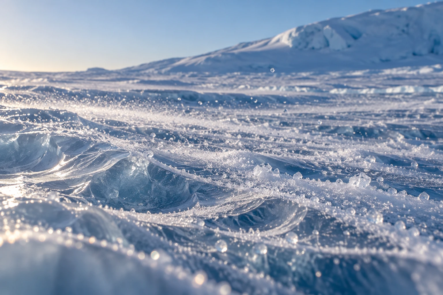
Small windblown snow crystals skimming a sculpted Antarctic ice surface
Snow traces only part of the near-surface flow; this illustration does not measure its speed.

Field research on the Ronne Polynya investigates heat exchange over one such coastal setting. As sea ice forms, much of its salt is rejected into the surrounding water. The consequences depend on the local ocean and ice conditions; an open patch in a photograph is not a direct measurement of dense-water production.

A 2025 modeling study focused partly on Cape Darnley shows why representing the wind is difficult. Changes in parameterized terrain drag and sea-ice roughness altered simulated near-surface winds. Finer grid spacing was not the only or necessarily dominant control. The surface through which a model exchanges momentum matters alongside the visible coastline.

Follow four arrows instead of one

Make four cards: heat lost from water, new ice formed, ice exported, and salt rejected. Arrange them in a plausible sequence, then add arrows showing feedback. An opening that remains visible may require continuous replacement of ice carried away by the wind. The opening’s area and the total ice manufactured there are different quantities.

Try an invented accounting example. Suppose an opening produces ten units of new ice and exports ten during one interval. Its local ice inventory can remain small even though production is substantial. On another day it produces only two and exports none; local coverage grows although production was lower. These units are deliberately abstract, not estimates of Antarctic conditions.

Now remove the wind card and add ocean heat. Some polynyas involve oceanic heat supply as well as mechanical ice removal, so the same visible opening need not identify the same balance. The correct question is which terms maintain this opening at this place and time.

This extends the slope story all the way to the sea. Cold air does not merely end its journey at the shoreline. Under appropriate conditions, its momentum and heat exchange can influence ice formation and the water left behind. A small open patch can be the surface sign of a busy production system.

A better way to read the landscape

On a topographic image, trace broad ice slopes, converging valleys, and the transition to flat shelf or sea. Then compare those features with a wind rose whose station, time span, and height are known. Ask whether the favored direction follows the local fall line or is offset, and whether strong events occur under particular large-scale weather patterns.

You do not need an expedition to appreciate the result. A continental ice sheet is not merely a passive white surface beneath the atmosphere. Through cooling and terrain, it helps organize the air immediately above it—and the resulting wind gives the shape of the ice a powerful, moving expression.

Sources and a next step

Continue exploring art, ideas, and unexpected connections at Incoprea.
The Atmosphere Has Tides You Can Find in a Barometer

A barometer is usually treated as a weather-change detector: pressure falls as a storm approaches, then rises behind it. But hidden within the irregular weather is a repeating signal tied to the solar day. The atmosphere has tides.

They are not simply ocean tides moved upward. Much of the atmospheric tidal response is driven by periodic solar heating. Daily patterns of absorption and heating excite global-scale waves in pressure, temperature, density, and wind.

Conceptual mixed-media artwork of an unnumbered brass barometer against a curved day-night Earth and translucent atmospheric bands.
Conceptual artwork of atmospheric pressure tides. The instrument face and colored air bands are illustrative, not data.

Heating can drive a planet-sized rhythm

As Earth rotates, the solar heating pattern moves relative to the ground. Water vapor, ozone, clouds, and other processes distribute that heating through the atmosphere. The response includes components with a 24-hour period and a 12-hour period, called diurnal and semidiurnal tides.

NCAR’s Global Scale Wave Model description explains how modeled tidal forcing includes solar absorption by water vapor and ozone and how background winds, temperature, and dissipation influence the response. The atmosphere is not expanding and contracting as one simple balloon.

Gravitational atmospheric tides also exist, but they should not be confused with the dominant thermally driven components discussed here. A shared word points to a periodic planetary response, not necessarily the same forcing mechanism in air and sea.

Twice a day is not twice as much sunshine

A daily forcing can be decomposed into harmonics. Its shape need not be a perfect sine wave; the atmosphere’s own wave structure and response determine which components become important at different heights and latitudes. A semidiurnal pressure signal therefore does not require the Sun to rise twice.

NCAR’s explanation of the diurnal tide also illustrates that different heating contributions can have different phases and partly cancel. Adding two drivers is not always equivalent to simply making the same oscillation larger.

This makes a useful analogy with music: two repeating contributions can reinforce or reduce one another depending on timing. The atmosphere is not literally a musical instrument with one fixed note, but phase is a physical quantity that affects the sum.

A pressure record contains several stories

At the surface, the familiar semidiurnal pressure tide is especially recognizable in tropical averages. Weather systems, local thermal effects, and instrument behavior can obscure it in a single day’s trace. A repeated pattern becomes clearer when many days are aligned by time and averaged.

Research on thermal tides in the tropical Atlantic examines surface pressure and related wind and precipitation patterns. The scientific interest includes the spatial structure, not merely the existence of a twice-daily wobble.

A weather app may show sea-level-adjusted pressure rather than the pressure actually measured at the station. Those products answer different questions. For a local analysis, first identify the variable, sampling interval, station altitude, and any corrections instead of combining unlike numbers.

A small home-data investigation

If you already have a stable electronic barometer or a public station series, gather several weeks of regular readings. Keep the sensor at a fixed height and temperature setting as far as possible, record missing intervals, and retain the unaltered data. Do not move it between a desk and an upstairs window mid-experiment.

  1. Plot each day against local clock time to look for repeated structure.
  2. Check whether daylight-saving changes or time-zone conversions create a shift.
  3. Subtract each day’s mean as a simple exploratory step, while noting that it does not remove every weather trend.
  4. Average by hour and compare the result with the spread among days.
  5. Repeat for different subsets, rather than trusting one attractive average.

The procedure is exploratory. It does not isolate a pure migrating solar tide, and sensor temperature sensitivity or regular indoor pressure changes could imitate a daily rhythm. If the pattern disappears when you remove a few days, that is useful evidence about its robustness.

Sampling can manufacture a rhythm

Suppose a hypothetical pressure signal repeats every 12 hours. Sampling only once daily always visits nearly the same phase; sampling every 12 hours can do the same. Neither schedule adequately shows the rise and fall. More frequent sampling reveals the shape, while careful timekeeping preserves its phase.

This is an original sampling example rather than a statement about a particular station. It illustrates why a long list of observations can still fail to resolve a periodic process. Duration and sampling interval must be chosen together.

Weather-driven changes also require care. A strong multiday trend can leak into an average or spectral estimate, especially with gaps. A frequency peak is a clue to investigate, not automatic proof of the physical source you hoped to find.

Keep the daily curves as well as their average. A repeating mean can be produced by a consistent small signal or by a few large excursions that happened at similar times. Compare the median hourly pattern and the spread if your tools allow it. If they tell a different story, investigate rather than selecting the prettier curve. The point is to find a stable relationship in the observations, not to make a household instrument reproduce a textbook diagram.

Which clock did the average use?

A repeating solar response is easiest to compare when the time coordinate follows the Sun consistently. Local civil time includes political time zones and seasonal clock changes. Local solar time follows longitude and the apparent daily solar cycle. The two can differ enough to shift a small average peak.

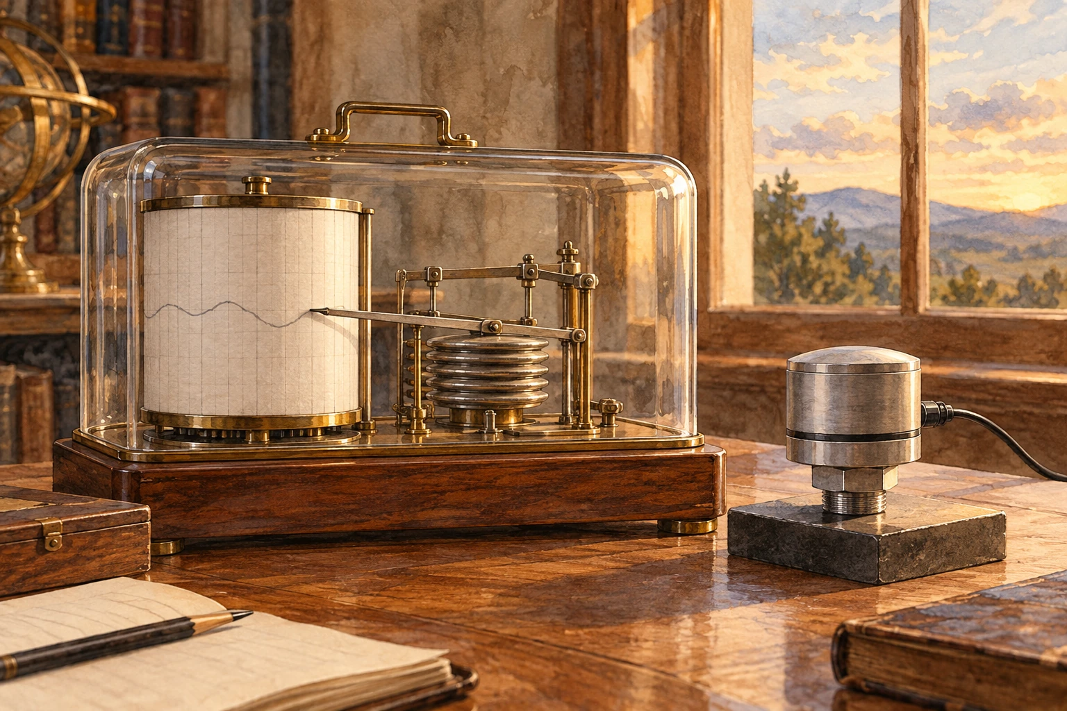
Mechanical barograph and modern pressure sensor on an observatory desk
Instrument study; the faint paper trace is illustrative, not a pressure dataset.

The Global Scale Wave Model documentation expresses tidal phases in local solar hours. The HAO description of migrating and nonmigrating tides adds another distinction: a daily period at one station does not uniquely establish how the global pattern travels in longitude. Multiple spatial samples are needed to identify that structure.

Fold an invented atmosphere

The demonstration below combines a 12-hour sinusoid with a weather-like variation and an optional observation-time offset. It is not a fitted station record. Its daily curves show how an individual day can conceal a small periodic component, while the hourly mean can expose it.

Fold an invented atmosphere

Compare daily curves and a mean with clock offsets and weather-like variation.

Open this activity in its own window.

First remove the extra variation and inspect the two peaks per day. Then restore it and increase the number of days. Predict whether the average should become more recognizable. The example’s added variations have a chosen mathematical form and are not a full model of weather; averaging real records does not guarantee that every unwanted component cancels.

Now shift the clock by one hour. The physical synthetic signal is unchanged, but its reported peak time moves. Next imagine joining half the record from one clock convention to half from another without documenting the switch. A sharp feature can become broader or weaker in the combined average.

Keep a copy of the daily curves beside the mean. A result that appears only after averaging might reflect a stable small rhythm, but it could also reflect uneven sampling or a repeated local schedule. Looking at subsets helps expose such alternatives. The strongest pattern is one whose phase and amplitude survive reasonable changes to the selected dates.

Finally write “solar tide candidate” beside the average rather than simply “solar tide.” Demonstrating a periodic component is one stage; identifying its source and global wave structure is another. The model turns a timekeeping nuisance into a useful lesson: a small planetary signal can be real, while a careless clock still tells the wrong story about when it arrived.

The tide grows into the upper atmosphere

Atmospheric tides can propagate upward and influence winds in the thin upper atmosphere. Their amplitudes and phases evolve as density, background flow, and dissipation change. NASA-supported work combining satellite observations and modeling investigates the migrating diurnal tide across the mesosphere and lower thermosphere.

NASA’s ICON findings connect upper-atmospheric winds and tides with electric fields in the ionosphere. Lower-atmosphere processes can thus influence a region commonly associated only with space weather.

The connection does not mean that one household pressure fluctuation predicts a satellite disturbance. It reveals a shared, vertically coupled atmosphere whose processes span scales far beyond the instrument on your table.

A barometer’s gentle repeat can be easy to overlook beside a storm’s dramatic plunge. Averaging patiently changes the view. The apparently noisy record begins to carry a regular planetary rhythm, made by sunlight and motion rather than by a visible tide line on a shore.

Sources and a next step

Continue exploring art, ideas, and unexpected connections at Incoprea.

Wednesday, October 14, 2026

Noctilucent Clouds: Ice That Catches Sunlight After Dusk

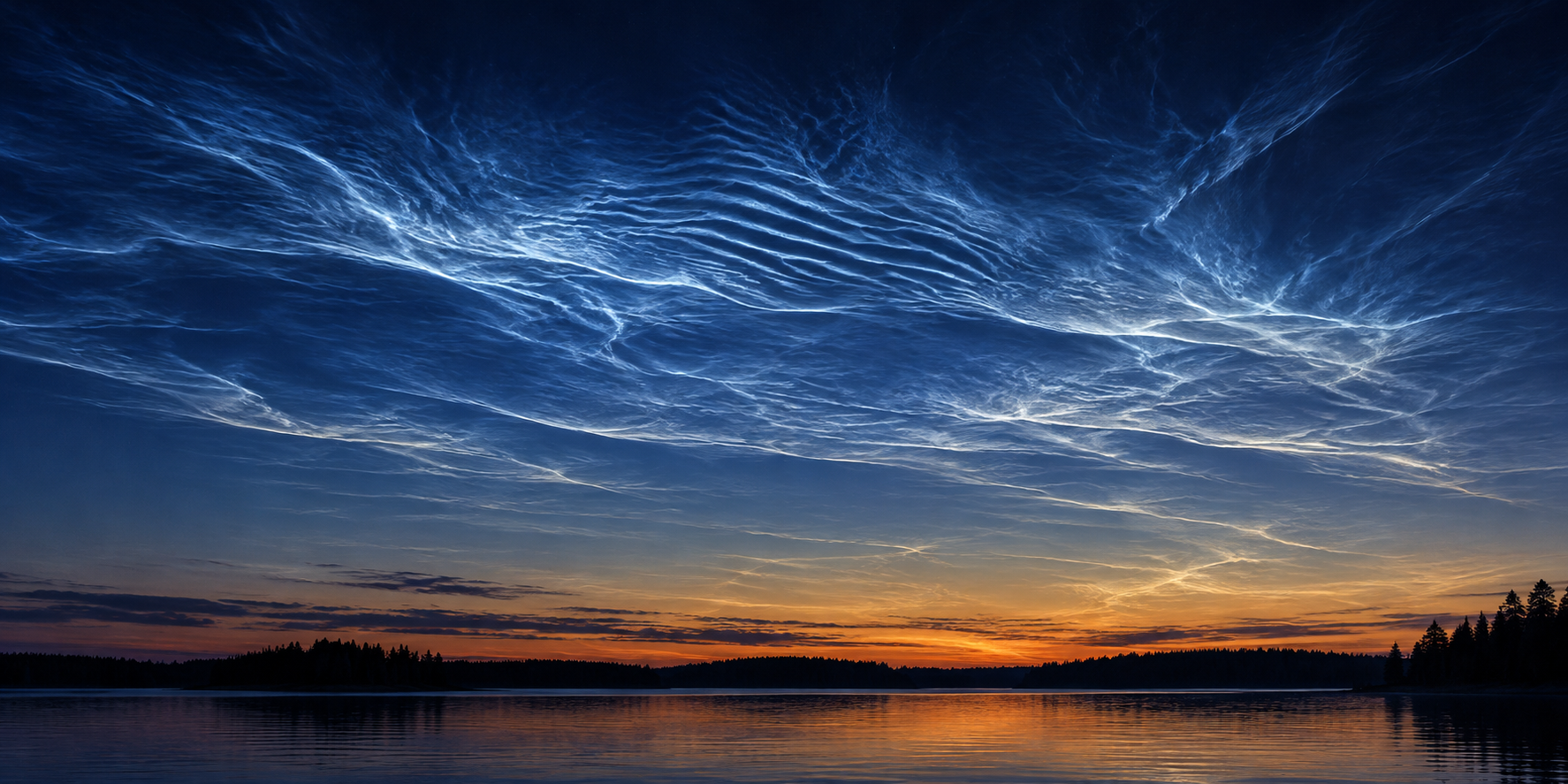
Silver-blue rippled clouds shine in a dark twilight sky over a silhouetted lake shore.
An idealized twilight view of noctilucent clouds, rather than a recorded sighting at a named place and time.

The landscape has darkened, ordinary clouds have turned grey, and then a fine blue-white lattice appears high in the twilight sky. Noctilucent clouds can look as if they produce their own light. Their name means night-shining, but their brightness comes from sunlight that still reaches their extraordinary altitude.

They occupy a different atmospheric neighborhood from the clouds that deliver rain. Understanding their height changes the apparent paradox: the observer can be in Earth's shadow while a thin cloud far above remains illuminated.

An unusually high place for water ice

Noctilucent clouds, also called polar mesospheric clouds, form near the top of the mesosphere. NASA places them roughly 76 to 85 kilometers above Earth's surface. That is far above the ordinary weather-cloud layer.

At those heights, the air is extremely thin and water is scarce. Under sufficiently cold conditions, tiny ice crystals can form. Sunlight reflected by the crystals gives the clouds their pale blue and silvery appearance.

The clouds are often associated with high latitudes during late spring and summer. That can seem backward: why would an ice cloud favor summer? The upper atmosphere has its own circulation and temperature behavior. The mesosphere can be particularly cold during the local summer, even while the surface is enjoying long, warmer days.

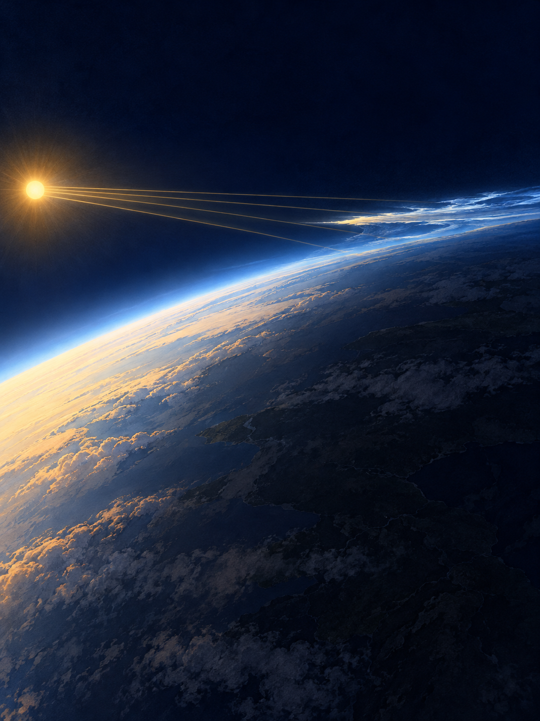
A schematic curved Earth lies partly in shadow while high clouds remain illuminated by sunlight.
Schematic twilight illumination with exaggerated cloud height and simplified light paths; the Sun and Earth are not shown to scale.

Sunset is a boundary moving through height

Picture a tall building at evening. Its upper floors can remain in sunlight after the street below has fallen into shadow. Earth's curved shadow creates an analogous geometry on a much larger scale: the observer's local sunset does not mean that every layer overhead has lost direct sunlight at the same moment.

Now place ordinary weather clouds and mesospheric ice at their different heights. After sunset, low cloud can become dark while sufficiently high ice is still illuminated. The contrast is especially noticeable because the sky behind the high cloud has dimmed. The cloud need not generate light of its own to appear striking against that background.

The analogy is limited by scale and geometry. It explains how a higher object can retain sunlight; it does not reproduce the full atmosphere, Earth's curvature or the scattering properties of ice. The schematic therefore exaggerates heights so that the relationship is readable. Do not estimate a real cloud's altitude by measuring the picture with a ruler.

A little material from space

Ice needs suitable starting material on which to form. NASA's AIM mission helped establish the role of very small particles called meteoric smoke, produced as material from space burns up in the atmosphere.

The term “smoke” does not mean a visible plume hanging above a meteor. It refers to tiny residual particles that become part of the upper atmosphere's chemistry and cloud formation. A familiar-looking ripple of ice can therefore include a connection to incoming extraterrestrial material.

This is one reason the clouds interest researchers beyond their beauty. Their formation depends on temperature, water vapor, particles, and atmospheric motion acting together.

What to put in an evening observation note

Begin with the time, viewing direction and a description of the structure. Are there thin ripples, a veil or bright bands? Note whether lower clouds are dark at the same time. Record nearby artificial light and haze, which can change contrast and create misleading bright patches. A sequence over several minutes can show changes that a single selected frame hides.

Color alone is a weak identification test. Cameras can shift a scene's color balance, and a bright image may result from a long exposure. The useful question is whether the timing, direction, texture and illumination geometry fit together. Compare the observation with NASA's documented images and animation instead of trying to match a particularly saturated picture.

The small ice crystals introduce a second kind of scale. The visible ripples describe organization across a large area, while the light is scattered by particles far smaller than anything you can resolve by eye. The meteor-derived material acts at that smaller scale by supplying sites around which ice can form. A cloud's broad pattern does not display the shape of individual grains.

This is also why a dramatic sighting cannot by itself establish a long-term change. A seasonal survey must consider when and where observers looked, what conditions allowed a view, and whether instruments or reporting habits changed. Your careful note can be a useful observation without having to carry a claim about an entire trend. The immediate puzzle is already rich: exceptionally cold summer air, scarce water, meteoric particles and sunlight surviving above a darkened ground all have to meet in the same place.

The sky is a connected system

AIM observations revealed relationships between different layers of the atmosphere and helped scientists study waves and circulation. Conditions lower down can influence events much higher up, and changes in one polar region can be linked with changes in the other.

Researchers also examine how cloud occurrence relates to long-term changes in water vapor and temperature. A single striking evening is an observation, however, not a diagnosis of the entire climate system. Establishing a trend requires consistent measurements over time.

See or hear more: See NASA's noctilucent-cloud animation.

Sources and further reading: NASA: Polar Mesospheric Clouds · NASA: Meteor Smoke Makes Strange Clouds · NASA: Taking AIM—10 science highlights

Famous Last Meals is now in paperback — stories, history and 25 recipes

Famous Last Meals: Stories, History, and Recipes is now available in paperback on Amazon. The illustrated collection brings together 23 his...