Showing posts with label Geology. Show all posts

Friday, October 23, 2026

Fulgurites: The Brief Lightning Strike That Leaves a Glass Archive

In a specimen drawer, a fulgurite may look like an unpromising root: rough, branching and coated with grains. A broken end reveals the surprise. Inside is glass, sometimes lining an irregular hollow passage. The object records an electrical event by preserving what happened to the ground.
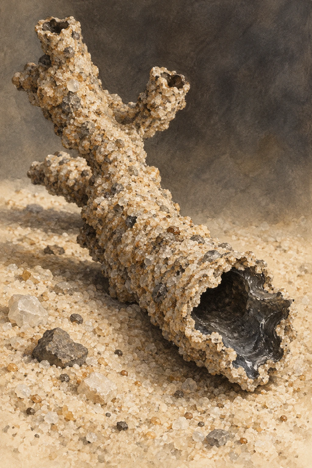
A rough branching hollow glass tube lies in pale sand, its broken end revealing a darker glossy interior.
A specimen-inspired sand fulgurite. The branching tube and granular surface convey one form; clay and rock fulgurites can look quite different.

Cloud-to-ground lightning can heat suitable material rapidly enough to melt part of it. Rapid cooling then arrests that melt as glass. The result depends on the material struck, how current travels through it, and how much energy is transferred over time. A fulgurite is therefore a physical record with local conditions built into it.

There is more than one kind of lightning glass

The familiar hollow sand tube is only one member of the family. A classification study by Pasek and colleagues distinguishes forms made in sand, clay, caliche and rock. Sand examples can have thin glass walls, while clay-rich targets can produce much thicker, melt-rich structures. Rock fulgurites may occur as glass associated with unmelted surrounding rock.

This variety changes how a specimen should be read. A thick wall is not automatically evidence of a stronger strike than a thin wall from a different substrate. The starting mixture’s mineralogy and physical arrangement also affect melting, heat transfer and the pathway available to current.

A strike has a duration as well as a peak

Experiments designed around realistic lightning discharges separated a short high-current impulse from a longer continuing-current phase. In those tests, the impulse alone produced limited melting; adding continuing current allowed fulgurite bodies to form in the tested materials.

The lesson is not that one laboratory result describes every strike. It is that a peak value cannot tell the whole energy story. A brief enormous current and a lower current sustained for longer can transfer heat differently. Material composition, porosity and the contact between grains complicate that comparison further.
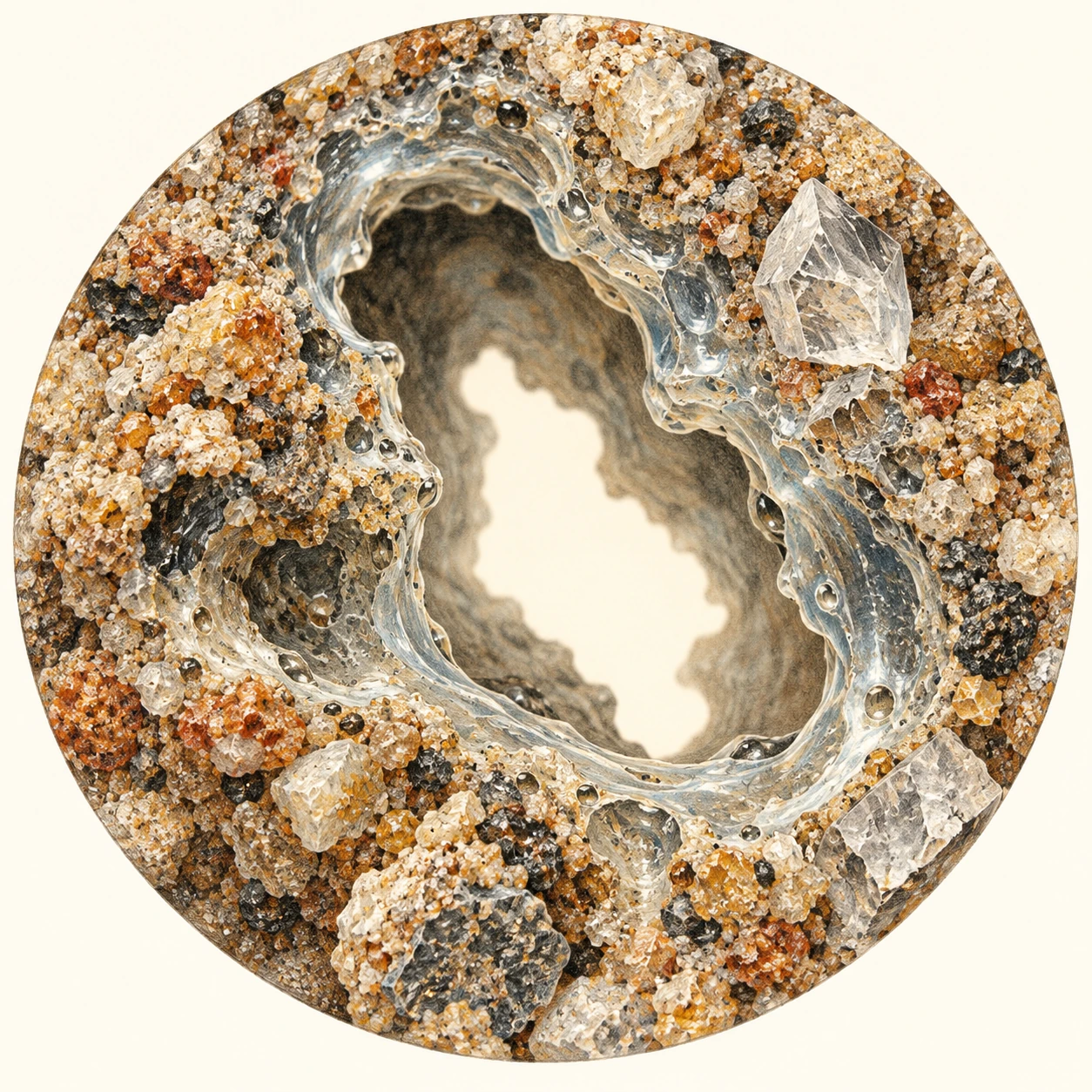
Interpretive section through a hollow tube with a glassy inner lining and rough fused grains outside.
A conceptual wall section separates cavity, glass and incompletely transformed grains. It is not calibrated microscopy or a measured specimen.

Read the wall before reading the weather

Use the conceptual section as a reading exercise. The central cavity, glassy lining and partly incorporated grains belong to different parts of the thermal history. They should not be treated as equally heated material with identical cooling rates.

  1. Trace the boundary. Where does smooth glass give way to recognizable grains? This is a question about material transformation, not just color.
  2. Keep the host in view. Compare the object with the sediment or rock in which it formed. An isolated tube loses information about that setting.
  3. Ask about measurement. Diameter, wall thickness, mineral identification and chemical analysis are different observations. A photograph cannot substitute for all four.
  4. Separate origin from reconstruction. Identifying a likely fulgurite is not the same as recovering the exact current waveform or the precise date of the storm.

This sequence is an original guide to evaluating evidence. It is not an identification key for an unknown object, and it does not ask readers to seek lightning strikes or excavate fragile specimens.

How much of the energy remains legible?

A 2016 study of Florida sand-mine fulgurites used morphology to estimate energy deposited per unit length. Its population had a geometric mean near one megajoule per metre under the study’s assumptions. That unit is important: it is not the total energy of an entire atmospheric flash.

The method connects a preserved material outcome with a model of heating and vaporization. Its usefulness rests on knowing the target and the assumptions. It should not become a universal ruler applied to every glass tube in a collection, especially when the host composition or preservation history is unknown.

The chemistry can change, too

Some fulgurites preserve reactions that require strongly reducing conditions. A study of a clay-rich Illinois fulgurite identified iron phosphide and examined how lightning could create chemically reduced phosphorus from more oxidized starting material.

The relevance to early-Earth chemistry is specific. Such a reaction offers a possible route to forms of phosphorus different from ordinary phosphate minerals. It does not show that a lightning strike created life, nor that every fulgurite has the same compounds. The researchers connected the outcome to the particular composition and reducing environment of their sample.

A fulgurite’s appeal is the mismatch between timescales. The heating event is brief; the fragile product may persist long enough to enter a geological collection. Reading it well means resisting a single dramatic story and instead following the glass, the grains and the chemical products separately.

Sources and further exploration

Explore all 80 new articles · Browse the complete illustrated collection

Keep exploring at Incoprea.

Sand Injectites: The Rock Layers That Broke Their Way Upward

Start with the beds. Thin layers run across the outcrop, one above another. Then a pale sandstone body cuts through them almost vertically, branches, and spreads sideways. If every sandstone is read as an old beach or river deposit, this one seems to violate its surroundings.

It may be an injectite: sand that was mobilized by fluid and pushed through fractures in material already present. The intrusion later became rock. Its geometry preserves movement through the sediment pile rather than straightforward deposition on top of it.

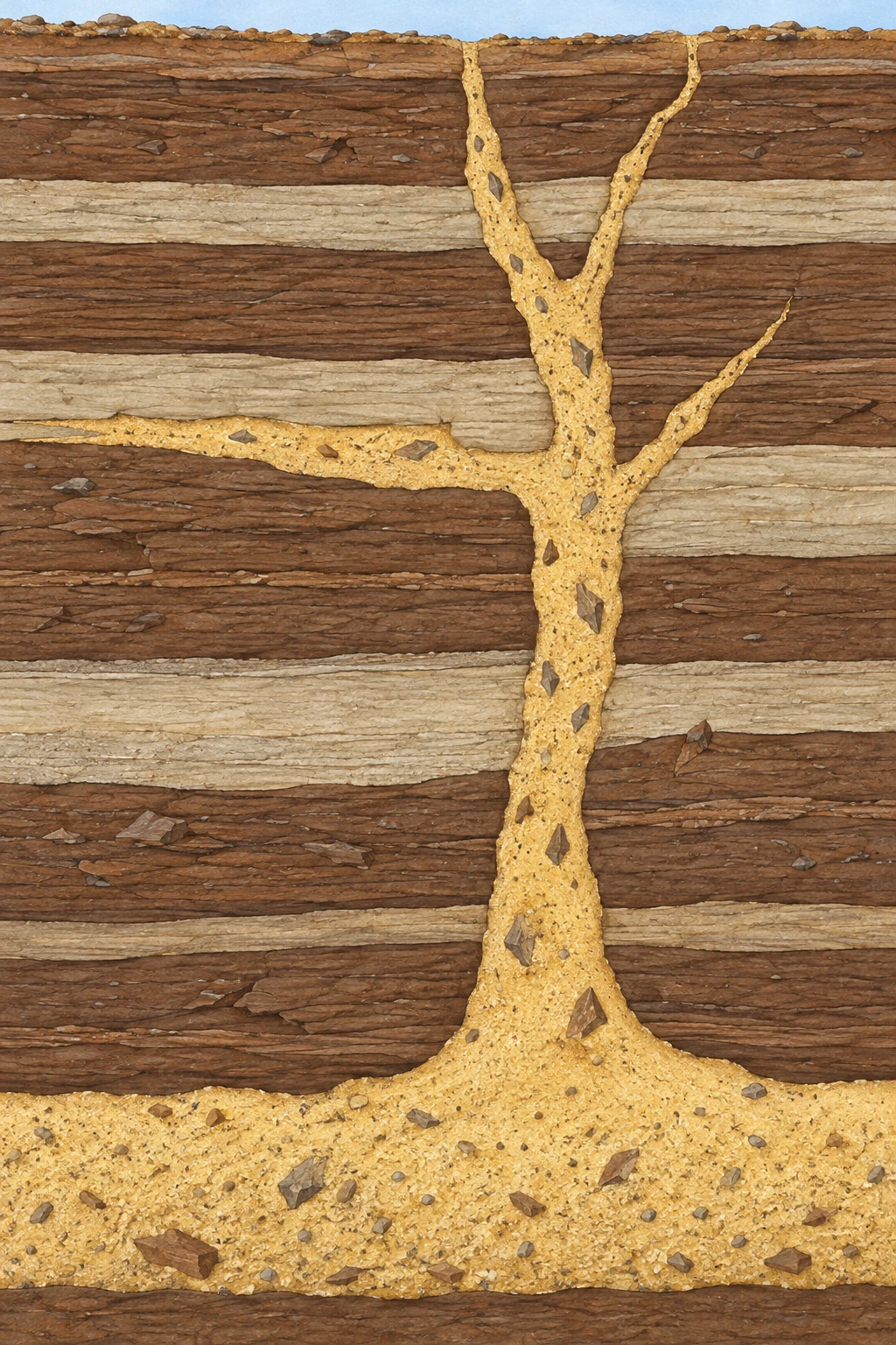
Pale sand-filled branches cut across dark horizontal beds, with a short lateral sheet and host fragments.
A conceptual injectite cuts older beds and follows one contact. Geometry, scale and fragments are illustrative; this is not a mapped natural exposure.

Pressure changes what a pile of grains can do

Buried sand is a framework of grains with fluid in the spaces between them. If pore-fluid pressure becomes high enough, it can reduce the load carried at grain contacts. When a route opens, moving fluid can entrain grains and carry them as a sand-rich mixture.

The host material matters. Fine-grained beds may restrict fluid escape, allowing overpressure to accumulate. Fractures can provide a new pathway. An injectite therefore records a relationship among sediment properties, pressure and failure; it is not simply a vein filled by sand falling into an open crack.

Experiments on forced folds and wing-like sand intrusions investigate how overpressure can deform a cover and create branching pathways. They help explain why intrusion and deformation can evolve together. Their two-dimensional apparatus is a controlled analogue, not a complete reproduction of a buried basin.

Read a small, imaginary outcrop

The following sequence is an original exercise. The drawing is conceptual, and the letters name relationships rather than a real locality. Imagine that a vertical pale body crosses three dark beds. A thin pale sheet follows one bed boundary, and angular fragments of dark material sit inside the pale body.

  1. Observation A: the dark layers end abruptly against the pale body. The cut layers existed before the material occupying that cross-cutting pathway.
  2. Observation B: pieces resembling the dark host occur inside the pale material. This is consistent with fragmentation and entrainment during intrusion, though their identity needs petrographic checking.
  3. Observation C: the pale body connects with a pale buried bed. That bed is a candidate sand source, not proof of a connection extending indefinitely outside the exposed face.
  4. Observation D: a later narrow crack cuts both host and injectite. Its relative age is younger than both.

Notice what is absent: an exact calendar date, flow speed and trigger. Relative order can be strong even when those quantities remain unknown. A cross-cutting relationship does more reliable work than a dramatic label such as “ancient sand explosion.”

The motion can change as the structure forms

In water-driven experiments by Ross and colleagues, injection and extrusion developed through stages including void formation, infiltration horizons, rupture and piping. Some pipes stayed in place; others migrated. Deposits produced by moving conduits could resemble material that had been fluidized more broadly.

This makes interpretation a genuine inverse problem. Researchers see a final arrangement and ask which histories could have produced it. Different processes sometimes leave overlapping signatures. Watching an experiment helps identify that ambiguity instead of assuming a preserved shape has only one possible origin.

The paper’s supporting-information section includes two short experimental videos. Their useful subject is the changing pathway: follow whether the active vent stays put and whether sand begins moving in neighboring regions. The laboratory dimensions belong to that apparatus, not to the natural structures it helps interpret.

A sandstone has texture as well as outline

A study of California’s Yellow Bank Creek complex examined grain-scale evidence and dewatering after emplacement. The authors interpreted a history involving water-rich and hydrocarbon-rich sand mixtures, followed by changing flow and compaction. Their account drew information from subtle fabrics that a distant landscape photograph would miss.

That case also explains why these structures attract attention below ground. A sand-filled pathway can connect permeable bodies across less permeable layers. Whether a specific structure acts as a conduit, a reservoir or a partly cemented barrier still depends on its continuity and later mineral history.

Three questions to take to a museum slab or a field photograph

Which contacts are actually visible? What feature establishes the proposed order of events? Which interpretation would change if the pale body were disconnected behind the exposed face? These questions keep a two-dimensional view from quietly becoming a complete underground map.

A good injectite story begins with something modest: sand is present where a depositional layer should not be. Following that inconsistency reveals a subsurface landscape in which fluids rearranged grains, broke boundaries and left the evidence in the rock.

Sources and further exploration

Explore all 80 new articles · Browse the complete illustrated collection

Keep exploring at Incoprea.
Thursday, October 22, 2026

Seismologists Can Make a Map From the Earth’s Background Murmur

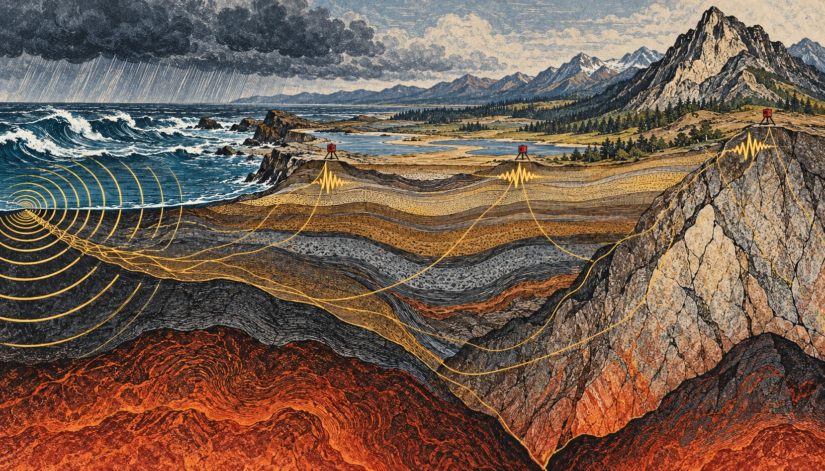
Linocut-style geological cross section from stormy coast to mountains, with small seismometers and conceptual vibration paths.
Conceptual illustration of ambient seismic noise and a sensor network; colors and paths are explanatory artwork, not tomography data.

If you could make the ground’s ordinary motion visible, a quiet day would stop looking quiet. Ocean waves, weather, traffic, and distant activity keep adding small vibrations. For an earthquake analyst these can be background. For another kind of seismology, the background is the experiment.

Ambient-noise tomography uses the continuous seismic wave field to estimate how waves travel between stations, then turns many such measurements into a model of Earth’s interior. It is a way of asking useful questions without waiting for a convenient earthquake to happen.

The ocean is part of the recording

A seismometer responds to ground motion, not merely earthquakes. USGS guidance on reading seismograms identifies background contributions from wind, human activity, and oceanic microseisms. A wiggly trace alone therefore does not establish an earthquake, much less tell you its magnitude or distance.

The ocean contribution is particularly striking. Waves interact with the solid Earth, and different mechanisms generate vibrations at different periods. The USGS account of microseisms distinguishes primary signals associated with the wave period from secondary signals associated with interactions between opposing wave components. A storm can help shake a seismometer far from the coast.

This does not mean that every visible wave drives a uniquely identifiable wiggle beneath your feet. A recording mixes many sources and propagation paths. The useful structure emerges statistically, after processing and enough observation time.

Two stations, one repeated question

Imagine two stations, A and B. Each records a long stretch of continuous motion. Shift one record relative to the other and compare them. At some time shifts, recurring wave energy is more consistently aligned than at others. Cross-correlation is the mathematical comparison that extracts this pattern.

Under suitable conditions, the correlation contains information resembling the response that would be recorded at one station if the other acted as a source. The virtual-source language is helpful, provided it is not taken literally: nobody has turned the first seismometer into a hammer. The wave field and the processing let researchers recover aspects of the path between them.

In the landmark 2005 California study by Shapiro and colleagues, a month of ambient noise from USArray stations yielded hundreds of surface-wave travel measurements. The resulting images distinguished major sedimentary basins from the faster igneous cores of mountain ranges. That is a concrete demonstration of the method, not a promise that one month is sufficient in every region.

From travel time to a map

Travel time is an integrated clue. A wave can cross several kinds of material before arriving. One measurement cannot say exactly which part of the path was slow. Many crossing paths help constrain where the slower and faster regions lie.

Picture trying to locate a traffic jam from journey times on overlapping bus routes. A slow trip might have several explanations; a whole network helps narrow them. The analogy stops at the physics, but it captures the inverse problem: infer an unseen distribution from its accumulated effect on things that passed through it.

Different surface-wave periods also respond to different depth ranges. Combining their behavior helps construct depth-dependent models. The result is a seismic-velocity model, not a literal photograph, and a velocity anomaly does not have only one possible geological cause.

A small calculation to make the ambiguity visible

Suppose two hypothetical paths are each 120 kilometers long. In a simple uniform model, a wave speed of 3 kilometers per second gives a 40-second travel time. At 2.5 kilometers per second, it takes 48 seconds. The eight-second difference is easy to see in this idealized arithmetic.

Now divide the slower route into two 60-kilometer sections. One might be fast and the other slow, yet their combined journey time could match a different, more uniform route. That is why a single average speed cannot locate a buried boundary. Additional paths and independent constraints provide the resolving power.

These are invented round numbers for understanding travel time, not measurements of California or an earthquake prediction. Real surface waves are dispersive, and researchers estimate quantities appropriate to the wave packet and method rather than applying this elementary model unmodified.

What survives when amplitude is thrown away?

There is an initially surprising experiment inside noise processing: replace positive samples with +1 and negative samples with −1. A huge pulse and a tiny positive wiggle now have the same value. This one-bit normalization deliberately removes much of the amplitude information before the records are compared.

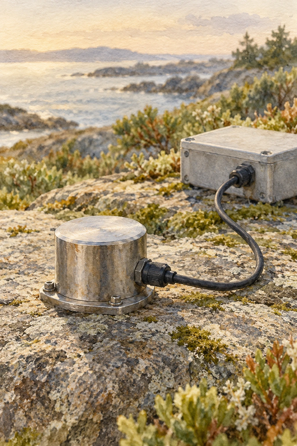
Small cylindrical ground-motion sensor resting on a prepared stone surface
Illustrative sensor study; the activity below uses invented numerical records.

The original study “One-bit noise correlation” investigates why useful correlation structure can survive that transformation under specified statistical conditions. It does not claim that discarding amplitude preserves every property of every recording. The point is that a treatment designed for timing information can have a different purpose from a treatment designed to measure physical amplitude.

Bensen and colleagues’ processing study places preparation, correlation, dispersion measurement, and quality control in one chain. Its emphasis on repeatability is helpful: an appealing correlation peak is less convincing if small changes in the selected days move it unpredictably.

Slide two invented records

The model below contains short numerical sequences rather than Earth observations. Slide one record across the other and compare the products of overlapping values. At a favorable shift, related features align. Add a single oversized outlier and watch how strongly an ordinary product sum responds. Switch to sign-only values and the outlier loses its numerical dominance.

Slide two invented records

Compare raw products and sign-only correlation with an oversized outlier.

Open this activity in its own window.

This is a demonstration of arithmetic, not a virtual seismology laboratory. The sequences are deterministic, the edges reduce overlap, and a short toy peak is not a travel-time measurement. Real records need instrument correction, appropriate filtering, much longer averaging, and tests of the noise field and processing choices.

Before moving a control, predict which result will change most when the outlier is enabled. Then ask a second question: what useful information did the sign-only version remove? If you wanted calibrated ground-motion amplitudes, losing the scale would be a serious cost. If a large transient dominated an estimate intended to emphasize persistent timing structure, reducing its influence could be useful.

That trade gives the word “cleaning” a more exact meaning. A cleaned record has been altered for a stated question. Keep the transformation attached to the result, so that a robust timing measurement is never casually retold as an untouched amplitude observation.

When the background changes

The noise sources do not surround a network evenly or remain constant through the seasons. That matters. USGS research on correlation amplitudes explicitly addresses how source distribution and attenuation influence the result. Reliable travel-time information does not automatically make every amplitude equally simple to interpret.

Time-lapse monitoring adds another challenge: a changed correlation can reflect a changed medium, changed noise illumination, or processing and instrument effects. Research on volcanic seismic interferometry explores how repeating measurements can track changes, but such monitoring must separate these possibilities. An interesting velocity variation alone is not a forecast with a date attached.

Listen with your eyes

Open a public seismogram through the USGS reading guide. Find the time markings and check how the trace is scaled. Before naming a wiggle, ask whether several stations recorded it, whether the timing fits a traveling event, and whether the background level changed. You are practicing observation rather than diagnosing a hazard.

The remarkable shift is intellectual as much as technical. “Noise” names a relationship between a signal and a question. Change the question, add the right network, and keep the assumptions visible, and the ground’s restless background can reveal structure that an isolated dramatic event would miss.

Resolution belongs on the map

Draw ten lines crossing a square, with most of them clustered along its left edge. You now have many paths but poor coverage of the right side. Adding a hundred nearly identical left-side lines will not solve the imbalance. A tomographic network has an analogous problem: measurement count and spatial resolving power are related, but they are not interchangeable.

This is why a convincing velocity image needs information about station geometry, path coverage, uncertainty, and recovery tests. A visually smooth color transition might be a feature of the inversion’s regularization rather than a sharp geological boundary. The appropriate question is not simply whether the map looks detailed, but which sizes and locations of structure the available observations can actually distinguish.

Sources and a next step

Continue exploring art, ideas, and unexpected connections at Incoprea.

Summer Ice in a Boulder Field: The Mountain’s Natural Cold Store

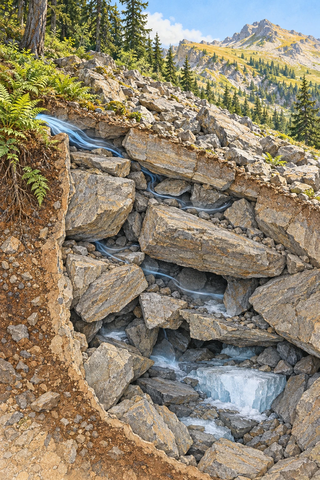
Colored-pencil cutaway of a summer talus slope with air spaces, small deep ice pockets, and cool air at a low opening.
Conceptual talus cutaway, not a surveyed site. Ice distribution and airflow are illustrative possibilities rather than measured conditions.

On a hot day, a small opening between boulders can breathe surprisingly cold air. In some mountain rock piles, winter’s cold is stored below the sunlit surface, and ice can persist into the warmer months. The surprise is not an exception to thermodynamics. It is thermodynamics operating through a complicated arrangement of stone, air, water, and time.

Talus is accumulated rock debris below a slope or cliff. Its interconnected spaces can create a thermal environment very different from the air a meter above it. But there is no single “natural refrigerator” mechanism that explains every cold boulder field.

A rock pile contains an air network

Large blocks can leave open voids through which air moves. Their arrangement controls ventilation, while the rock mass stores heat or cold and limits the speed of conductive temperature change. Snow and ice add insulation and phase-change energy to the system.

The National Park Service’s talus-cave guide explains how mechanically accumulated boulders can leave interconnected spaces. Such cavities differ in origin from limestone caves dissolved by water. A talus cave also does not automatically contain perennial ice.

That last point matters in photographs. A dark opening among rocks establishes a void, not its annual temperature regime. You need measurements through the seasons to know whether ice persists, forms seasonally, or is absent despite cool summer air.

Winter can charge the cold store

In a ventilated slope, density differences between outside and internal air can drive circulation. During cold conditions, cold air may enter lower openings while warmer internal air escapes higher up. The resulting chimney effect can cool parts of the debris mass.

Numerical research on convective heat transport in permafrost talus investigates how airflow changes the thermal regime. Geometry and permeability are not minor details: if fine material blocks the pores or ice seals routes, the ventilation changes.

Summer circulation and cold-air outflow can then expose the stored cold at low vents. The seasonally changing flow is not simply a fan that runs identically all year. The direction and strength depend on the contrast between the slope interior and the outside atmosphere.

Ice adds a thermal delay

Melting ice requires energy without immediately raising the ice-water mixture’s temperature. This latent heat can buffer warming. Rock shade and restricted air exchange further affect how quickly summer heat reaches the interior.

A useful idealized calculation uses ice’s latent heat of fusion, about 334 kilojoules per kilogram. Melting 100 kilograms requires roughly 33.4 megajoules, even before warming the meltwater. At a hypothetical net heat input of 100 watts, that energy alone corresponds to nearly 3.9 days.

Those numbers are not a prediction for a real vent. Natural heat exchange varies with airflow, water, geometry, and weather. The calculation simply explains why a modest ice reservoir can delay a temperature response rather than disappearing the moment the air becomes warm.

A specific place, with a specific season

The Nature Conservancy’s Ice Mountain Preserve in West Virginia describes a sandstone talus that produces cool air from openings near its base. Its account notes winter ice that can remain into summer and a local plant community associated with the cool conditions.

This is a place-based example, not proof that all cold vents preserve ice year-round. A research abstract on Ice Mountain airflow explicitly notes that year-round ice persistence is not essential to summer cold-air flow. Stored cold in the rock and the pattern of air exchange belong in the explanation too.

It also changes how the landscape should be treated. Moving a boulder, blocking an opening, or repeatedly entering a small refuge can alter airflow or damage sensitive vegetation. An inviting cool spot may be part of a fragile microclimate.

Imagine replacing the coarse open blocks with tightly packed fine gravel while leaving the slope and outside weather unchanged. The altered air pathways would change ventilation. Now restore the blocks but add an insulating snow cover over selected openings. That changes the boundary conditions again. These hypothetical alterations show why the size distribution of debris and the seasonal snow pattern belong in a thermal study rather than being treated as background scenery.

Several mechanisms can coexist

Ventilation is not the only possible heat-transfer route. Conduction from adjoining rock walls, snow distribution, water movement, and ice formation can influence the thermal pattern. Modeling of rock-wall and talus heat flow examines a conductive contribution while discussing its interaction with ventilation.

The distinction between demonstrating a possible process in a model and establishing its dominance at a field site is essential. A process can be physically real yet small compared with another process under the conditions actually observed.

Different regions also have different boundary conditions. A snow-covered Alpine talus, a shaded Appalachian boulder field, and a lava-tube cold trap should not be folded into one story merely because all can preserve summer ice.

An observation plan that keeps the slope intact

From an established path or authorized guided visit, compare air temperature in shade near a vent with shaded air away from it. Use the same sensor and allow it to equilibrate. Record time, weather, recent rainfall, and the exact measurement height without placing equipment inside unstable voids.

Repeat across seasons if access is permitted. A single cool reading demonstrates a local contrast at that moment; it does not show the annual minimum, the presence of permafrost, or the volume of buried ice. Photographs should document the observation position so a later comparison uses the same setting.

Avoid digging, moving stones, entering unassessed cavities, or treating old visitor instructions as current access permission. The scientifically useful activity is a careful comparison, not an attempt to open the refrigerator door.

A refuge can buffer a day without escaping a changing climate

For an animal living among rocks, the temperature below the surface can matter more than a regional weather-station average. American pikas use talus and related rocky spaces as thermal refuges. The spaces can reduce the extremes an animal experiences, but “buffered” does not mean permanently insulated from long-term change.

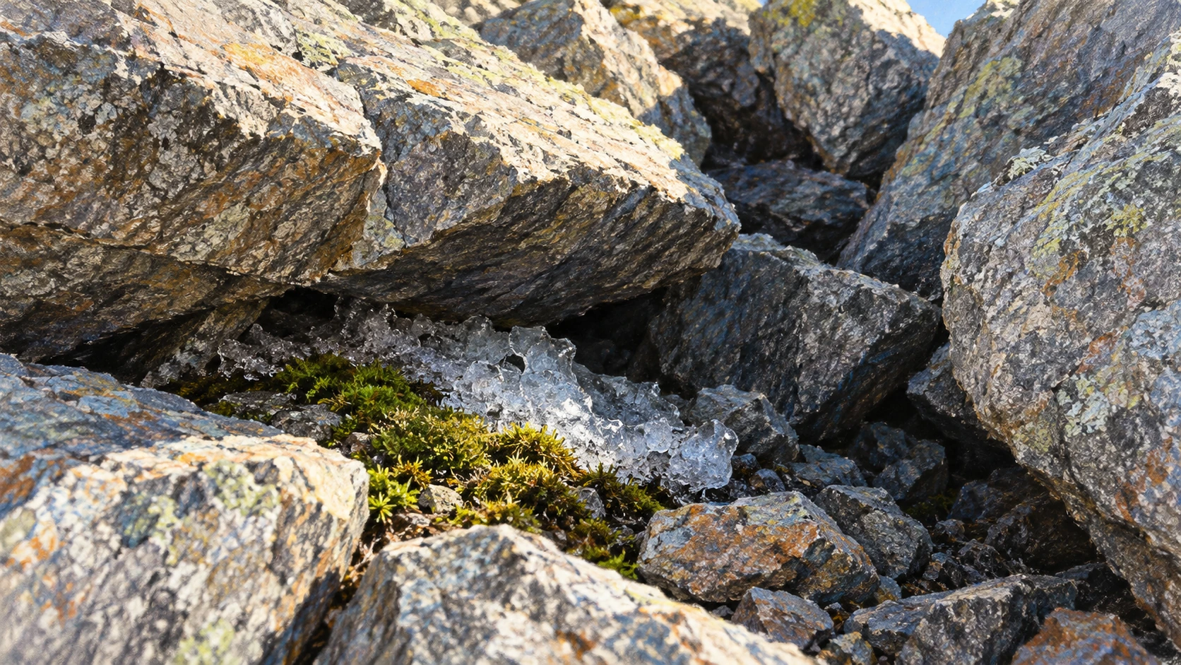
Shaded boulder interstices sheltering a small ice patch and moss
Conceptual cool microhabitat; ice in the picture is not evidence of year-round ice at a real site.

Research comparing subsurface pika microrefuges examined different rock substrates and populations. It asks about the actual environments available to an animal, rather than assigning all talus one temperature. A shaded opening, a deeper matrix, and the exposed surface can be different habitats within the same mapped patch.

Monk and Ray’s 2022 study revisited a Southern Rockies site with rare 1963–1964 measurements. Its historical comparison suggested substantial subsurface warming, particularly in winter, while explicitly discussing differences in sensor placement and methods. This is evidence from one carefully examined setting, not a measured trend for every cold boulder field.

Read four curves, not one cool number

Imagine a hypothetical hot-day record. Exposed rock reaches 35°C, shaded free air 25°C, a shallow void 18°C, and a deeper void 12°C. Those invented values describe a strong local gradient. They do not establish the annual average, winter conditions, or the presence of ice.

Now give all four curves a different winter history. Snow may alter insulation and ventilation; an exposed surface may experience cold extremes that do not reach the deeper space in the same way. A summer-only survey would miss that part of the refuge’s function.

On paper, make a two-by-two grid: surface and subsurface across the top, summer and winter down the side. Write the measurement you would need in each box. Then add a second year rather than assuming the first was typical. The exercise turns “a cool habitat” into a testable seasonal description.

Finally separate temperature from habitat quality. Food nearby, access between shelter and forage, predators, moisture, and the amount of usable space can matter too. A particularly cold crack does not automatically provide everything an animal needs. The refuge is a relationship between an organism and a landscape, not simply the lowest number on a thermometer.

The mountain’s thermal memory remains fascinating. This ecological view makes it more consequential: a hidden delay in heat transfer can change the conditions available to living things, while still responding to changes in the wider environment.

The mountain keeps a delayed weather record

What feels like impossible summer cold is a lag between external weather and internal heat storage. The talus has a memory because air routes, rock, snow, and ice exchange energy on different timescales. The cold breath at its base is the moment that hidden seasonal history meets your hand.

Sources and a next step

Continue exploring art, ideas, and unexpected connections at Incoprea.

Columnar Basalt: How a Cooling Crack Learns to Turn

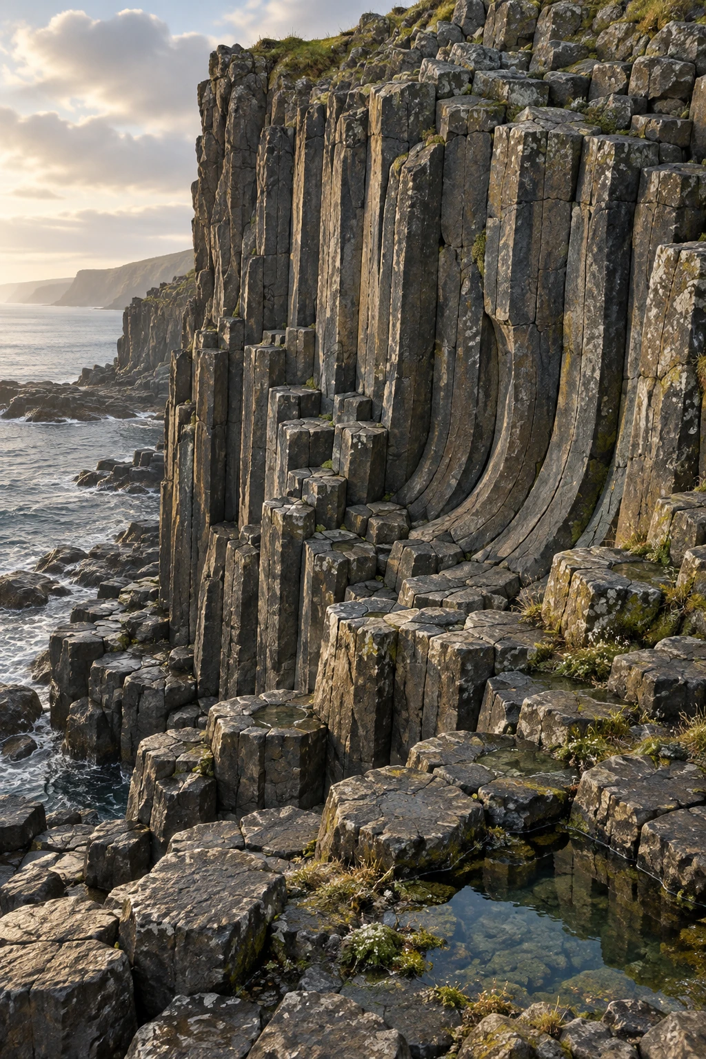
Ink-and-gouache illustration of a weathered basalt cliff with polygonal column tops, long joints, and gently curving columns.
Geological illustration inspired by columnar jointing, not a photograph or mapped reconstruction of a named outcrop.

A basalt cliff can resemble a bundle of stone pencils. From above, the pencil ends form polygons; from the side, their joints can run in long parallel lines or bend into fans. The geometry looks designed, yet it records the advance of cooling and fracture through hot rock.

The columns are not crystals grown to giant size. They are pieces of rock separated by a three-dimensional joint network. Understanding that distinction opens a more interesting question: how does a crack pattern keep organizing itself as it moves deeper?

Solid rock still has cooling to do

Lava loses heat from its margins, solidifies, and continues to contract as solid rock cools. If the surrounding material prevents free contraction, tensile stress develops. Fractures release some of that stress.

The USGS explanation of columnar jointing describes cracks advancing inward from cooling surfaces in discrete events. The visible columns are the geometry left behind as this fracture front migrates.

The word “cooling” should not suggest that molten lava simply freezes into ready-made hexagonal rods. Solidification, further thermal contraction, stress buildup, and crack propagation are related but distinguishable stages. The joints tell a history after the rock acquired enough strength to fracture.

Why the columns point the way they do

Columns commonly extend roughly perpendicular to cooling surfaces. If the cooling boundary is horizontal, the result may be vertical columns. If the boundary curves, the joints can change orientation and produce fanning or bent forms.

The National Park Service overview includes columnar jointing in several volcanic rock settings, not only basalt. A column’s orientation therefore needs to be read against its geological context rather than assumed to point vertically in the original flow.

A useful field question is where heat could escape. Was the rock against a valley wall, beneath a cooled upper crust, over cooler ground, or in contact with water or ice? The joint pattern can constrain that story, though several processes may have influenced it.

Why approximately hexagonal?

As neighboring cracks interact and the front advances, the pattern can reorganize. Mature networks often have many six-sided columns, but five- and seven-sided sections and other irregularities remain. A natural outcrop is not a perfect honeycomb.

Goehring and colleagues’ study of basalt joint scaling compares field observations, laboratory analogs, and thermal models. It treats the geometry as a dynamic fracture problem, including how crack spacing relates to the advancing front.

This is more useful than saying “nature prefers hexagons” and stopping. That slogan names a familiar outcome but does not identify the material, stress, transport, or evolving boundary conditions that produce it.

A kitchen material helps investigate a volcanic pattern

Drying starch slurries can form columnar fracture patterns. Water loss plays an analogous role to cooling-induced contraction, allowing researchers to control conditions and observe structures too slow or inaccessible to watch easily in a lava flow.

Laboratory experiments on columnar-joint scaling examine how the drying conditions influence column size. The analogy is not an assertion that lava and starch have identical properties. It isolates a shared problem of shrinkage, transport, and a moving fracture front.

Laboratory control also helps distinguish correlation from mechanism. If a changed drying rate alters the pattern under controlled conditions, researchers can compare that response with expectations from field cooling histories. The analog gains value through the match of relevant physics, not the visual similarity alone.

Read the joints as a sequence

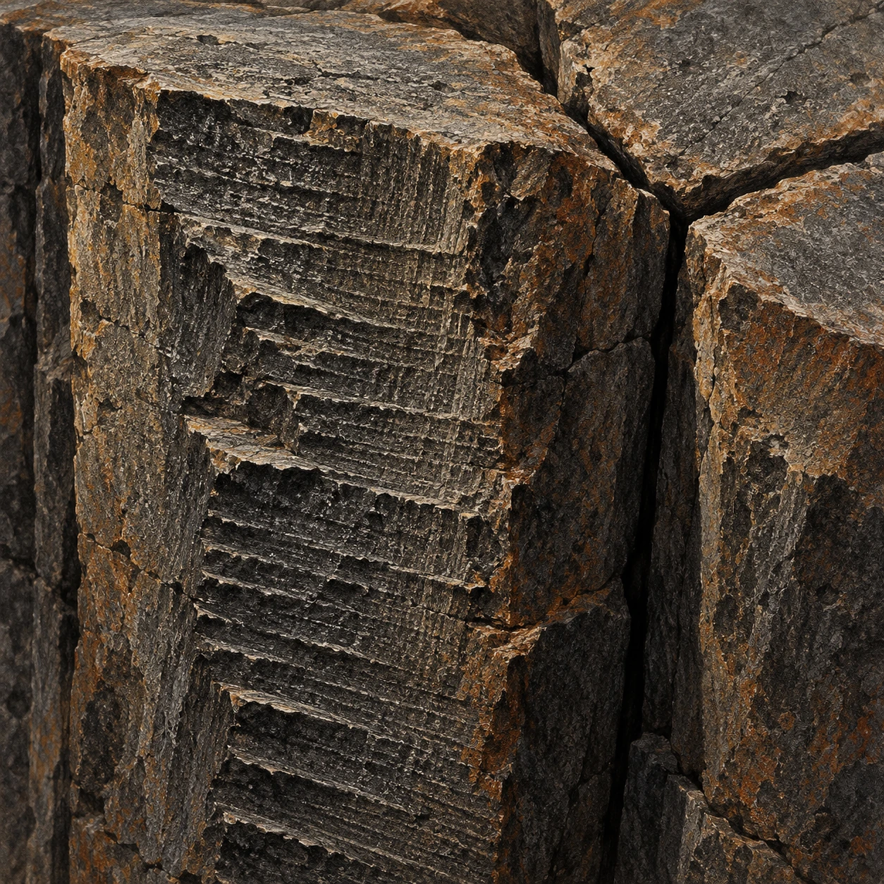
Basalt joint faces with fine stepped ridges beside a three-way junction
Illustrative fracture-detail study; striae and joint shapes are not measurements from a named outcrop.

First look: where do three cracks meet? At a T-shaped junction, one crack can terminate against another. At a roughly Y-shaped junction, three directions meet at angles closer to 120 degrees. Goehring’s study of evolving fracture patterns explains how repeated small adjustments can turn a more rectilinear network toward a more hexagonal one. The result records an evolving process, not a shape selected in one instantaneous decision.

Second look: what is written on a side? A column face can preserve striae associated with incremental crack advance. Instead of treating the side as a smooth rod, look for small repeated steps. They offer another scale of evidence: a long column can have formed through many short fracture events.

Third look: was the material still liquid? Lamur and colleagues’ laboratory investigation combined thermal and mechanical measurements to examine when basalt fails during cooling. Their tested material fractured below its solidus, supporting joint formation in solid rock that still had considerable heat to lose. The experimental temperature range belongs to that material and setup, not to every columnar outcrop.

A photograph can become a fracture notebook

Choose a published close-up in either study. Make three passes over it. In the first, mark candidate junction types. In the second, mark possible striae without assigning a temperature. In the third, note which features you cannot distinguish because of weathering, lighting, or the viewing angle.

Then try a useful question: could an apparent small step be a later weathering feature rather than a primary fracture mark? A photograph may not decide. A fresh fracture surface, matching marks on neighboring faces, or a broader field relationship would add information. Keeping alternatives does not make the notebook indecisive; it states what evidence would improve it.

Why is a perfect hexagon count an incomplete answer?

It describes a cross section but loses the sequence through depth. Two exposures with similar side counts can differ in junction development, striae spacing, cooling boundaries, and later erosion. Pattern statistics become more informative when paired with the rock’s three-dimensional context.

The added close-up deliberately changes the article’s scale. The cliff gives the impression of a great architectural whole. A junction and a stepped face bring the explanation back to local crack interactions. Understanding how those small events continue through the rock makes the larger order more interesting than a slogan about nature liking six sides.

Count the sides without forcing the answer

Use a clearly photographed horizontal exposure of column tops. Select a region before counting, then record the number of sides for every complete visible polygon in it. Put ambiguous or partly hidden polygons in a separate category.

If you choose only the most symmetrical columns, your result will overstate the regularity. If you count a fractured or eroded edge as an original side, you may distort the distribution in another direction. A simple tally becomes a lesson in sampling and classification.

Do not break rock or climb an unstable face for a better view. Existing public photographs can support the exercise, and protected sites often have designated viewpoints. The scientific question is the pattern’s variability, not the acquisition of a souvenir.

Two textures in one flow

A regular colonnade may sit beneath a more irregular, closely fractured entablature. USGS descriptions of Columbia River basalt interiors show these contrasting joint patterns. Different cooling histories, including water involvement, can help create differences within one lava body.

That means a cliff’s upper and lower sections need not be separate eruptions simply because their fractures look different. Conversely, identifying a single flow requires more evidence than matching column shapes. Contacts, composition, textures, and regional mapping belong in the interpretation.

You can also test how much the viewpoint changes the apparent geometry. A vertical face reveals column length and joint direction but may hide the polygonal cross sections. A top surface reveals side counts but says less about how the columns bend below. Combine both views before describing the whole outcrop. A photograph that makes the rock look like an orderly bundle may conceal substantial variation just outside the chosen frame.

A cooling history with uncertainty attached

A broad rule links faster front advance with finer spacing in appropriate regimes, but an exact column diameter is not a universal thermometer or stopwatch. Composition, geometry, heat transport, and the sequence of cooling events complicate the relationship.

Try drawing the same rock body with three different cooling boundaries: flat top, curved valley side, and irregular water contact. Sketch columns normal to each. The exercise makes the fanning shapes less mysterious while leaving the quantitative reconstruction for actual data and models.

The stone pencils are therefore records of movement rather than symbols of stillness. Their rock has stopped glowing, but the joint network preserves a front that once advanced, adjusted, and released stress one crack at a time.

Sources and a next step

Continue exploring art, ideas, and unexpected connections at Incoprea.

Zircon Clocks: A Tiny Crystal Can Keep More Than One Geological Date

A zircon grain can be smaller than a pinhead and older than the rock now carrying it. It may have crystallized in one geological episode, survived erosion, entered a sediment, and acquired a younger rim during later heating. Calling it a tiny clock is useful, provided the clock is allowed to have a history.

Uranium-lead geochronology measures isotopic ratios and interprets them in that history. The result is not simply “the age of the stone.” A good question asks which event, in which part of the grain, a particular date represents.

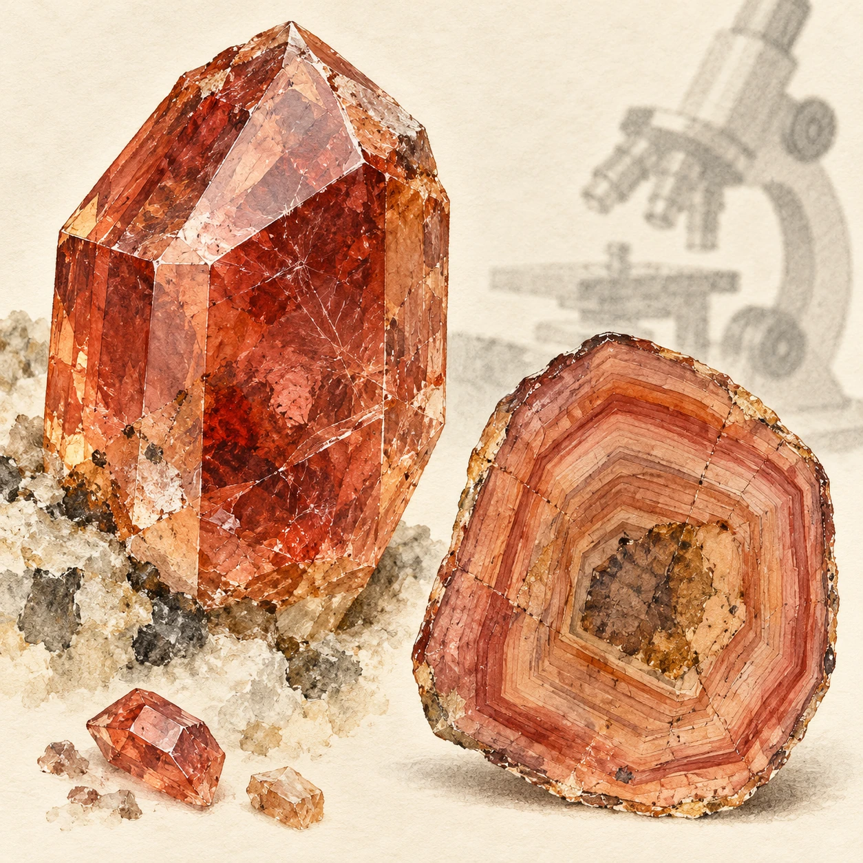
Enlarged watercolor zircon crystal beside a conceptual polished section showing an older core and younger growth zones.
Mineral study and conceptual growth-zone section. It is not a microscope image, isotope map, or dated specimen.

Why zircon keeps appearing in geological timelines

Zircon’s crystal structure can incorporate uranium while generally incorporating little lead when it grows. Radioactive uranium then produces lead through known decay chains. The mineral is also resistant enough to survive many later geological processes.

The American Museum of Natural History’s zircon chronology guide explains how the mineral records multiple episodes. Its durability is both an advantage and a complication: an inherited grain can preserve an older event inside a younger host.

That is why a very old zircon in sandstone does not make the sandstone equally old. The sand grain had to exist before it was deposited. Its crystallization age can constrain the sediment’s history, but it is not automatically the deposition age.

Two related isotope clocks

Two uranium decay systems are especially useful: uranium-238 to lead-206 and uranium-235 to lead-207. Their different decay constants provide related age estimates that can be compared. Under an ideal closed-system history, the ratios agree on an age.

UCL’s geochronology teaching chapter introduces the concordia diagram, whose curve represents agreement between these systems over time. A measured point is accompanied by uncertainty, often shown as an ellipse. The visual test is more careful than deciding whether a dot looks close to a line.

“Closed system” means the relevant parents and daughters have been retained in the way assumed by the model. It is a testable geological and analytical proposition, not permission to ignore alteration, lead loss, or non-radiogenic lead.

When a grain does not tell one date

A zircon can contain an old core and younger growth zones. Measuring across both may mix information. Imaging the polished grain helps researchers choose analysis locations and connect isotope measurements with visible textures.

Yellowstone Science’s discussion of zircon dating illustrates how age measurements fit geological questions and how populations of detrital grains can help trace sediment sources. The analysis is strongest when the grain’s context survives the journey from field sample to published plot.

Lead loss can move a result away from concordia. In suitable cases, a set of discordant analyses can help constrain an older formation event and a later disturbance. But a fitted line is not a universal decoder for every complex history. More than one episode, mixed zones, or unsuitable assumptions can make a simple interpretation misleading.

A three-age thought experiment

Imagine a hypothetical crystal core formed 1,500 million years ago. It erodes into sediment deposited 500 million years ago, then grows a metamorphic rim 200 million years ago. A core analysis and a rim analysis can both be valid while giving very different dates.

Now ask four questions. When did the core crystallize? When was the sediment deposited? When did metamorphism affect it? When was the present outcrop exposed? The two zircon analyses directly address only some of those questions. Other observations and methods must fill the gaps.

These invented ages are not a real sample. They show why “the dates disagree” is often the wrong first conclusion. Different measurements may have successfully dated different events.

The instrument’s scale changes the question

Spatially resolved methods can target small zones, while dissolving selected material for isotope-dilution analysis can offer a different precision and averaging strategy. Each approach trades spatial information, analytical uncertainty, sample preparation, and potential sources of bias differently.

The London Geochronology Centre lists several isotope systems and analytical capabilities. Seeing multiple methods together helps dispel the idea of one universal rock-age machine. Laboratories choose techniques to match the material and event of interest.

A date with small analytical error can still be interpreted incorrectly. Precision describes the measurement’s spread under its analytical framework. Geological accuracy also depends on identifying the event, screening disturbance, and accounting for shared systematic uncertainties.

For one more check, put the core and rim dates on a timeline together with the host rock’s mapped relationships. An older grain enclosed in a younger deposit is geometrically possible; a proposed event sequence that places deposition before its supposed source crystal formed needs reconsideration. The exercise is not an independent date, but it tests whether the interpretation respects the order implied by the evidence. Numbers become more informative when their geological verbs—grew, eroded, settled, reheated—are written beside them.

Sometimes the preparation is part of the question

A zircon’s resistance does not make it indestructible. Radioactive decay can damage its crystal structure, and damaged domains can be more susceptible to losing lead. A measured ratio then reflects both production and subsequent history. Before interpreting an unexpectedly young date as a young growth event, a laboratory has to investigate whether the system remained closed.

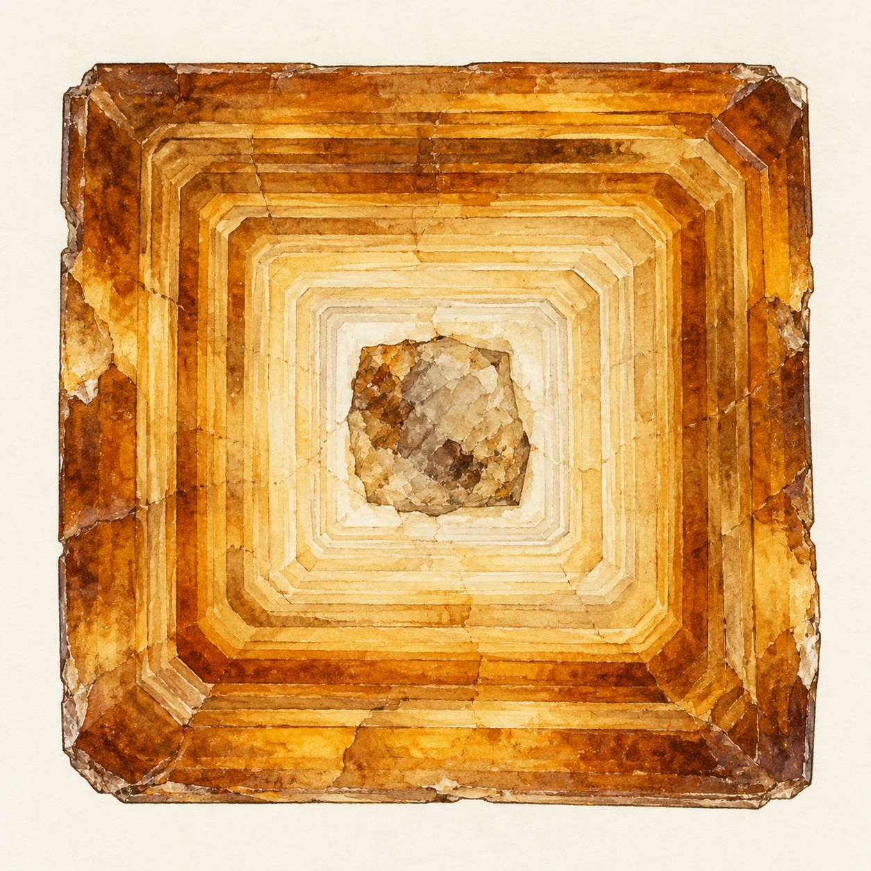
An enlarged square zircon cross section with angular growth zones around an irregular core
Conceptual tetragonal mineral-zoning section, enlarged and interpretive; no dates or microscope measurements are shown.

In a Caetano caldera study by Watts and colleagues, unexpectedly young SIMS dates motivated a comparison of chemically abraded and untreated zircon. Chemical abrasion is a preparation approach intended to remove susceptible material. This is not a way to make every grain give the desired age; it is an intervention whose effects must be documented and tested.

A 2026 paired-method study of detrital zircon illustrates a related strategy. After screening sandstone grains with laser-ablation measurements, researchers selected some apparently youngest grains for more precise follow-up by chemical-abrasion isotope-dilution thermal-ionization mass spectrometry. The same geological question can require a broad survey and a smaller, more detailed investigation.

Which grain would you investigate next?

Suppose an invented sandstone dataset contains most grain dates near 150 million years, a small cluster near 120 million, and one at 90 million. The lone youngest analysis could matter enormously for an attempted maximum depositional age. It could also be the result that most needs checking.

Choose between three next steps: repeat a measurement in the same zone, image the grain and target another zone, or apply a preparation and analysis method that tests a lead-loss explanation. There is no universal winner. Your choice depends on whether the first measurement’s spatial context, uncertainty, and disturbance behavior are already known.

Write what each step could resolve. A repeated spot can test reproducibility without eliminating a shared bias. Imaging can reveal growth or alteration textures without independently dating them. A different preparation and analytical approach can test a mechanism, while changing what portion of the grain survives to be measured.

Does the youngest number automatically date deposition?

No. A reliable youngest detrital crystallization date can provide a maximum-age constraint: the sediment must have been deposited after that grain formed. It may have been deposited much later. Disturbance can produce misleadingly young apparent dates, and a youngest population needs a geological as well as statistical interpretation.

Now change the example so that the 90-million-year result is a well-characterized younger rim instead of an unexplained spot. You have changed the event being dated, not merely improved the decimal places. The preparation, zone, and geological verb belong beside the number.

This view makes laboratory work less mysterious. An instrument does not deliver a historical verdict on its own. Investigators choose which material to preserve, which potential disturbance to test, and which independent relationships make the resulting interpretation credible.

Read an age table as a chain of evidence

  1. Find the sample’s rock type and field relationship.
  2. Check whether the analysis targeted a core, rim, or whole grain.
  3. Read which isotope ratio and correction method produced the date.
  4. Look for discordance criteria, uncertainty conventions, and excluded analyses.
  5. Compare the interpreted event with independent geological constraints.

This guide is for reading published work, not selecting favorable points until a desired age appears. Exclusions need a stated rationale, and uncertainty should be carried into the geological conclusion.

A USGS zircon and monazite report from Vermont offers an example of a documented multi-sample study. Rather than starting with its oldest number, inspect how samples, analyses, and interpretation are connected. The supporting table is part of the result.

The crystal is an archive, not a verdict

A dramatic “oldest material” headline can be an entry point, but the richer story is how a mineral preserves and sometimes edits evidence. Growth, transport, heating, damage, and measurement each leave their mark.

The reader gains more by following one grain’s sequence than by collecting superlative ages. Inside that small crystal, geological time is not a single label. It is a set of events that careful analysis can begin to separate.

Sources and a next step

Continue exploring art, ideas, and unexpected connections at Incoprea.

Luminescence Dating: The Clock That Starts When a Grain Loses the Light

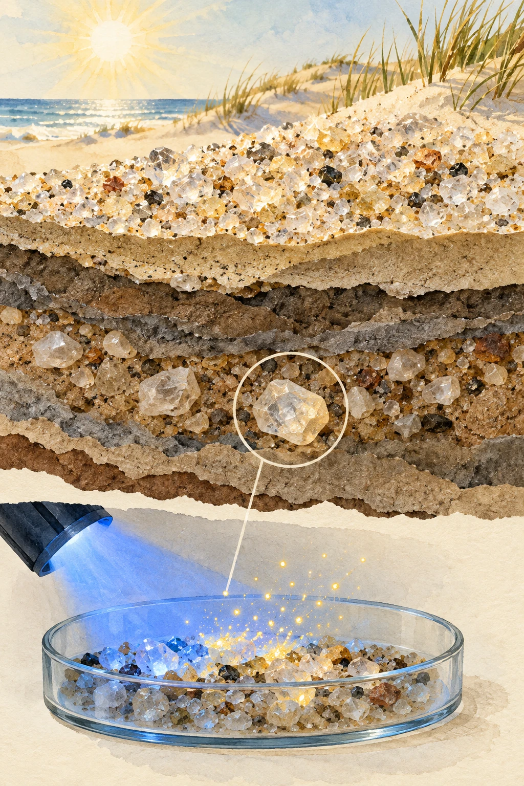
Watercolor collage of sunlit quartz sand, buried sediment grains, and a laboratory tray under conceptual blue stimulation light.
Conceptual illustration of luminescence dating. Gold specks visualize a stored signal; buried grains do not visibly glow this way.

A sand grain can carry a record of the last time it saw enough light. Bury it, and natural radiation gradually stores a signal in defects within its crystal structure. Bring it into a laboratory and stimulate it carefully, and the grain releases light that helps estimate the time since that reset.

Luminescence dating is therefore a different kind of geological clock from a mineral’s crystallization age. The quartz may be very old. The event being dated can be its much later exposure and burial.

What is stored?

Ionizing radiation from the surrounding environment and cosmic rays transfers energy to mineral grains. Some charge carriers become trapped at defects in the lattice. Suitable light or heat can release them, producing luminescence and reducing the stored signal.

The USGS Luminescence Dating Laboratory explains the age relationship: equivalent dose divided by dose rate. The principal minerals include quartz and potassium feldspar, and different stimulation procedures suit different materials and questions.

This is not a case of ordinary daylight becoming trapped as visible photons inside the sand. Radiation builds a charge-related signal, and later stimulation causes light emission. The distinction makes the clock’s resetting and accumulation easier to understand.

A dose is not yet a duration

Suppose a hypothetical sample yields an equivalent dose of 30 grays and an average environmental dose rate of 2 grays per thousand years. The simple age estimate is 15 thousand years. If the appropriate dose rate were instead 3 grays per thousand years, the same dose would imply 10 thousand years.

The calculation uses invented round numbers. It shows why measuring the laboratory signal is only half the problem. Researchers also need a defensible account of the radiation environment throughout burial, including moisture, surrounding radionuclides, overburden, and internal contributions where relevant.

A precise equivalent dose cannot rescue an inappropriate dose-rate history. Water can attenuate radiation, and changing burial conditions can alter the contribution from cosmic rays. The past environment becomes part of the age model.

Resetting is a physical event, not an assumption to hide

Sunlight exposure can bleach a grain’s signal before burial. Wind-blown sand may have a different exposure history from sediment moved rapidly in turbid floodwater. If some inherited signal remains, treating it as entirely new accumulation can make a burial age appear too old.

A USGS sampling guide emphasizes resetting, dose-rate characterization, and post-depositional mixing. It also explains why a sample must include light-safe material and material needed to characterize its radiation environment.

The dark tube in a field photograph is therefore not a theatrical laboratory precaution. Exposing the protected sample to sunlight can erase precisely the signal researchers hoped to measure. Sampling strategy is part of the evidence, not a separate logistical footnote.

One handful can contain several histories

Grains can be incompletely bleached, mixed after deposition, or respond differently during measurement. An average of many grains may conceal that variation. Single-grain or small-aliquot analysis can help characterize the distribution, while introducing its own practical and statistical challenges.

A guide to interpreting and reporting luminescence results discusses how suitable reporting connects the measurements with the geological interpretation. A lone age and error bar may be insufficient without information about dose distributions, selection, and the model used.

Some feldspar signals can fade anomalously, while some signals saturate at high doses. Different protocols address different limitations. There is no single maximum age that applies identically to all minerals, environments, and techniques.

Write the event on the sample label

Try this paper exercise. Draw three grains: one blown across a sunny dune and buried, one carried briefly in muddy water, and one mixed downward by a burrowing animal long after deposition. Write what event you hope to date beside each, then list what could prevent the clock from matching that event.

The sunny grain may offer favorable bleaching but still need a stable burial history. The flood grain may retain an old signal. The mixed grain may date a different episode than the surrounding layer. None of these sketches proves a sample unsuitable; they identify the questions a real analysis must test.

Now add a fourth object: fired pottery. Heat can reset a luminescence signal, so the relevant event may be firing rather than sunlight exposure. The age principle is related, but the sample and resetting mechanism change.

To see the effect of incomplete bleaching, return to the thirty-gray example. If six grays of that signal survived from an earlier history, only twenty-four grays accumulated after the intended reset. With the same two-gray-per-thousand-year dose rate, that simplified corrected duration would be twelve thousand years rather than fifteen. This is an accounting exercise, not a practical correction to apply without measurements. A laboratory must establish how the grains behave and which statistical model is appropriate; an assumed inherited value cannot be subtracted merely to make an age fit expectations.

How do you turn a faint light into an equivalent dose?

The laboratory does not read a burial duration from a grain’s brightness as though it were a watch dial. It compares the natural signal with responses produced by known laboratory doses. The comparison builds a dose-response curve and asks where the natural measurement falls on it.

Sand aliquot disc and closed sample tube in a dim red-lit laboratory
Illustrative sample-handling still life. Grains are not shown emitting visible light.

The single-aliquot regenerative-dose work of Murray and Wintle addresses a complication: a sample’s sensitivity can change during repeated treatment and measurement. A subsequent test dose provides a way to normalize that changing response. The point is a controlled comparison on the material, not an assumption that every measurement cycle has the same sensitivity.

Later tests using violet-stimulated quartz luminescence show why a protocol must be evaluated for the signal actually being used. A procedure that works well for one signal cannot simply inherit that credibility for another. Recovery of a known dose is a more demanding test than a smooth-looking curve alone.

A response curve with a difficult upper end

The toy below uses the invented relationship response = 1 − exp(−dose/50). Its values have no mineral calibration. Near the beginning, an extra dose changes the response substantially. Near saturation, a large extra dose makes a small difference. Choose a natural-response value and inspect the inferred dose.

Read an invented dose-response curve

Explore saturation and nonlinear uncertainty before making a time conversion.

Open this activity in its own window.

Compare a response of 0.2 with 0.8. Then change each by 0.02. The dose changes are not equal because the curve’s slope differs. This is why a small uncertainty in light output need not become a constant uncertainty in equivalent dose. Close to saturation, an apparently small measurement interval can span a much larger dose range.

The example leaves out background subtraction, sensitivity correction, recuperation, grain selection, and the details of stimulation. It does not estimate an actual sample age. After equivalent dose is determined, the environmental dose-rate history still has to connect that stored dose to time.

For a report-reading task, make three separate checks. First, was the natural response inside a well-characterized part of the growth curve? Second, did repeated or recovery tests support the protocol’s behavior? Third, did the dose rate describe the intended burial environment? Passing the first does not automatically pass the other two.

Finally imagine an ideal laboratory result for a grain that was never fully bleached before burial. The instrument can accurately measure its stored signal while the assumed resetting event remains wrong. Measurement quality and geological interpretation are connected responsibilities, and neither can do all the work of the other.

What a careful report should let you check

Four links between a number and a burial history
Report itemWhy it matters
Mineral and stimulation protocolDifferent signals have different behavior
Equivalent dose and its distributionReveals scatter and possible mixed histories
Dose-rate components and moisture assumptionsSets the conversion from stored dose to time
Stratigraphy and independent constraintsConnects the measured clock to the intended event

Geoff Duller’s guidance for English Heritage gives a detailed account of reporting and interpretation. USGS guidance for paleoseismic research shows how the method can address geological events where organic material for radiocarbon dating is absent or unsuitable.

Light can erase a clue and reveal another

The final laboratory glow is faint, but the history behind it is large: a grain’s last exposure, transport, burial, radiation environment, and later disturbance. The most useful question is not whether sand “remembers sunlight” perfectly. It is how well a particular mineral signal, sampled in a particular layer, records the event you want to understand.

Sources and a next step

Continue exploring art, ideas, and unexpected connections at Incoprea.

Cosmogenic Nuclides: Reading How Long a Rock Has Faced the Sky

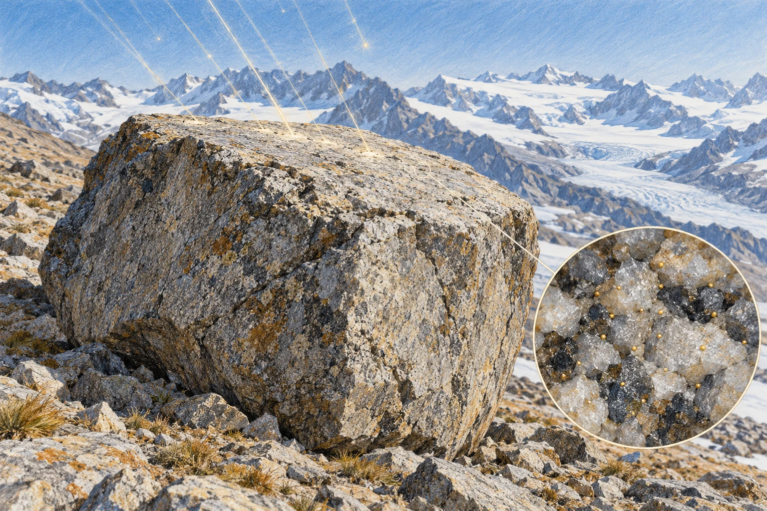
Colored-pencil alpine moraine boulder with faint conceptual particle tracks and a magnified surface-crystal detail.
Conceptual artwork of cosmogenic exposure. Particle tracks and isotope dots are visual metaphors, not visible features or measured data.

A glacier leaves a boulder on a ridge and retreats. The boulder’s exposed surface begins accumulating rare isotopes made by cosmic-ray interactions. Much later, a small rock sample can help estimate how long that surface has faced the sky.

Cosmogenic exposure dating is not the age of the boulder’s original rock. It is an interpretation of its near-surface history. A granite block can be hundreds of millions of years old while its present exposed face records only the most recent part of that story.

Space makes a small inventory in stone

High-energy cosmic particles generate secondary particles in the atmosphere and near-surface material. Nuclear interactions produce rare nuclides in minerals. Commonly used examples include beryllium-10 and aluminum-26 in quartz, though several other systems are available.

A USGS review of cosmogenic dating explains how measured concentrations, production rates, and decay behavior become tools for dating landforms and estimating erosion. The production is small, requiring sensitive chemical preparation and measurement.

The signal is strongest near the surface and changes with depth. It also depends on altitude, geomagnetic conditions, shielding, and the target mineral. A universal “atoms per year” value cannot be pasted onto every rock on Earth.

The simplest clock is a useful first model

If a stable nuclide accumulates at a constant rate P, begins with no inherited inventory, and is neither eroded nor shielded, its concentration N grows asP multiplied by time. Dividing N by P gives the exposure duration in that deliberately simple model.

For a radioactive nuclide, decay must also be included, and production and erosion can change. The point of the simple model is to expose the assumptions. Each term omitted from it becomes a possible reason the apparent exposure age differs from the landform event.

National Park Service research in the western Alaska Range connects the method with glacial deposits. A moraine’s chronology depends on selecting surfaces whose exposure is plausibly tied to the glacier’s retreat or the deposit’s stabilization.

Three ways the surface history can mislead

Inheritance: a rock already exposed before deposition can carry nuclides into its new setting. Interpreting the full inventory as newly accumulated can produce an apparent age older than the intended event.

Shielding: snow, sediment, water, surrounding topography, or temporary burial can reduce production. Treating an intermittently covered surface as continuously open can make the inferred duration too short.

Erosion or rotation: removing the nuclide-rich outer layer or turning a different face upward can reset part of the observable history. The rock is not a sealed counter that always keeps every event.

USGS work on Yosemite rock-fall deposits explicitly discusses inheritance, erosion, boulder rotation, fire-related spalling, and shielding. The complications are not objections discovered after the method was invented; they are central parts of sampling and interpretation.

A numerical thought experiment

Imagine a hypothetical nuclide produced at 10 atoms per gram per year under fixed conditions, with decay ignored over the example’s timescale. A concentration of 100,000 atoms per gram would imply 10,000 years in the simplest model.

If 20,000 atoms per gram were inherited before the target event, only 80,000 belong to the new exposure, implying 8,000 years under the same assumptions. If shielding reduced production during part of the history, a different correction would be needed. The same measured number can support different durations when the history changes.

These invented values illustrate the accounting, not the actual production rate for a specified mineral, latitude, or altitude. A real calculation uses calibrated scaling and propagates uncertainty rather than choosing round numbers.

Why field photographs matter to a laboratory date

Researchers record the boulder’s setting, stability, surface shape, sample thickness, surrounding horizon, and evidence for erosion or burial. A large stable top surface may be preferable to a loose edge that could have rotated recently.

A Yosemite account of investigating the El Capitan rock avalanche shows how carefully chosen boulders link a landscape question with laboratory analysis. The field interpretation determines what event the measurement can plausibly date.

An accelerator mass spectrometer can count a rare isotope with remarkable sensitivity. It cannot reconstruct an unrecorded snowbank or a boulder’s unnoticed overturning by itself. Better instruments do not make geological context optional.

Consider two neighbors on the same ridge: a stable boulder and one that overturned recently. Their underlying rock can have the same formation age, while their upward-facing surfaces carry very different recent exposure histories. Photographing only their present positions does not reveal the overturning date. Look instead for physical evidence of stability, weathering contrasts, and the relationship with surrounding sediment. This thought experiment shows why several samples from a landform are valuable without assuming that their mean must be the correct answer. Replication helps test a geological story; it does not remove the need to choose that story carefully.

More than one nuclide can reveal burial

Different nuclides have different production relationships and decay behavior. Measuring more than one can constrain exposure and burial histories that a single concentration leaves ambiguous. This is especially valuable when material has alternated between surface and shielded conditions.

Lamont-Doherty’s cosmogenic laboratory guide outlines several systems and applications. Its broader program shows that the same physical process can address glacier history, landscape erosion, and sediment transport, provided the model matches the question.

A buried surface can keep losing two clocks at different rates

The paired-nuclide idea becomes easier to grasp with a period when production nearly stops. If a previously exposed surface is deeply buried, radioactive nuclides already present continue to decay. A faster-decaying nuclide loses a larger fraction of its inventory than a slower one. Their ratio can therefore preserve information about the burial interval.

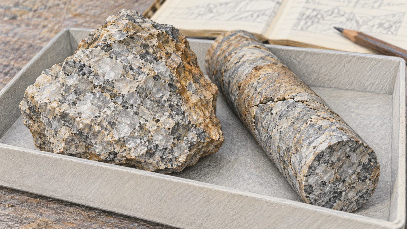
Quartz-rich rock and a slender bedrock core in a plain sample tray
Material study; these are not dated samples from Greenland or Salida.

The GreenDrill project’s explanation applies multiple nuclides to bedrock beneath Greenland’s ice. A rock currently hidden from the sky can retain evidence of an earlier exposure. The interpretation combines the inventory with production, shielding, erosion, and the ice-sheet history rather than treating burial as a perfect universal off switch.

A USGS data release for alluvial deposits near Salida offers a different real application. It separates aluminum-26 and beryllium-10 measurements from location information and interpreted burial-age results. The documented revision of the sampled unit’s geological identification is especially instructive: a laboratory result needs an accurate account of what deposit was sampled.

Let two invented nuclides decay

In this model, nuclide A has a half-life of one arbitrary time unit and B has a half-life of two. Both begin at an inventory of 100, with no new production and no loss except radioactive decay. After two units, A is 25 and B is 50. The A/B ratio has changed from 1 to 0.5.

Two invented burial clocks

Compare unequal half-lives and the importance of the initial ratio.

Open this activity in its own window.

Move the burial-duration control and predict which curve falls faster. Then double both initial inventories. Their absolute values change, but their ratio history is identical. Now change only the initial A/B ratio: the final ratio no longer provides a unique duration unless that initial relationship is known or constrained.

The arbitrary half-lives deliberately avoid masquerading as an exposure-age calculator for real isotopes. Real burial dating may include inherited inventories, continued production at depth, erosion, mixtures, and multiple exposure episodes. A clean curve here demonstrates only the mathematical effect of different decay rates.

For a final notebook exercise, draw three stages labeled exposed, buried, and exposed again. Mark production as high, low, or resumed, and leave the exact values unspecified. Ask which parts of that history a single final concentration cannot distinguish. Add a second nuclide and decide what extra constraint it provides.

The surprising archive is not only a surface that faced the sky. It is a surface whose subsequent absence from the sky changed the relationship between the clues it already carried.

Read the age population before the headline

If several boulders on one moraine yield different apparent ages, do not immediately average them into one confident date. Ask whether the scatter reflects measurement uncertainty, inherited exposure, delayed stabilization, erosion, or more than one landform episode.

A useful paper exercise is to draw five boulders and assign each a different complication. Decide what extra field evidence would help distinguish it. The goal is not to reject inconvenient data, but to make the geological explanation testable.

The exposure clock is remarkable because it reads a surface’s relationship with the sky. Its strongest results come from combining an extremely small isotope inventory with an unusually careful history of an ordinary-looking rock.

Sources and a next step

Continue exploring art, ideas, and unexpected connections at Incoprea.

Famous Last Meals is now in paperback — stories, history and 25 recipes

Famous Last Meals: Stories, History, and Recipes is now available in paperback on Amazon. The illustrated collection brings together 23 his...