Showing posts with label Physics. Show all posts

Sunday, October 25, 2026

The Diamonds in a Jet Are Pressure Finding Its Way Out

The exhaust behind a jet engine sometimes looks as though someone threaded bright diamonds onto a flame. The pattern can remain in roughly the same place while gas rushes through it. That combination is the first clue. The diamonds are not a string of solid objects or separate packages of fuel. They are a visible consequence of a repeating flow structure.

Conceptual view of a nozzle above a luminous exhaust plume with repeating diamond-shaped cells.
The illustrated exhaust plume shows repeating cells associated with shock diamonds.

NASA photographed this effect during maximum-afterburner testing of the X-59 research aircraft. Its official image account calls the shapes Mach diamonds, also known as shock diamonds. The photograph records a particular engine test on January 22, 2025. It is a good place to start because the image is real, its context is stated, and the attractive pattern does not have to carry an invented performance claim.

An aircraft does not need to travel at supersonic speed for gas in its exhaust to be supersonic. The relevant Mach number belongs to the local flow. A ground engine test can therefore show diamonds while the test stand and camera remain stationary. Keeping vehicle speed separate from exhaust speed prevents a photograph of a test from becoming a claim about flight.

A pressure mismatch does not vanish at the nozzle

A nozzle guides expanding gas toward its exit. The static pressure at that exit may differ from the pressure of the surrounding atmosphere. If exit pressure is higher, the jet is underexpanded: further expansion is available outside the nozzle. If exit pressure is lower, it is overexpanded relative to its surroundings and the external atmosphere initially compresses the jet. These terms compare pressures, not whether the engine looks powerful or weak.

In supersonic flow, adjustments take the form of waves and organized regions rather than the gentle pressure equalization familiar from slow air movement. The jet can expand too far, compress, then adjust again. Its boundary and internal wave pattern form a series of cells. The European Space Agency's plume explanation relates pressure mismatch to shock waves and expansion waves. Both underexpanded and overexpanded flows can produce shock-cell structures; the early part of the pattern differs.

Compression and expansion do different work on the flow

A shock wave is a very thin region across which flow properties change abruptly. In the ideal gas treatment used in introductory compressible-flow analysis, static pressure, density, and temperature rise across a shock. The flow loses total pressure. That last term is important: a shock is an irreversible adjustment. It is not a free compressor that increases all useful measures of pressure at once.

An oblique shock meets the flow at an angle. It turns the gas while changing its properties. NASA Glenn's account explicitly notes that oblique shocks can occur downstream of a nozzle when the expanded pressure differs from outside conditions. The textbook equations have assumptions, including a simplified gas model and defined flow geometry. They explain the structure without implying that one formula describes every hot, chemically reacting exhaust plume.

An expansion fan is different. The supersonic gas turns through a spread of small changes, with decreasing static pressure and increasing Mach number in the ideal treatment. NASA's centered expansion-fan explanation contrasts this with a shock. Alternating compression and expansion help create the repeating cells. An expansion does not simply undo a shock's loss of total pressure, even when the visible plume seems to repeat a symmetrical shape.

A standing pattern made from passing material

Think of a stationary wave in a fast stream. The shape can hold its place while new water continually passes through. Shock diamonds have a comparable distinction between material motion and pattern location, although their compressible-flow physics is very different. A gas parcel travels through successive regions; the whole diamond does not have to travel with that parcel. A long-exposure picture can make this separation especially easy to miss.

The visible brightness is also not a complete pressure map. Light emission depends on temperature, chemical species, combustion conditions, and the camera's wavelength response and exposure. Shock-related changes can help make some regions brighter, and afterburning can contribute in relevant plumes. A cold gas jet can have shock cells that need specialized optical methods to reveal. Conversely, a bright plume photograph alone cannot supply an exact pressure, temperature, or thrust for every bright patch.

Read the image carefully
ObservationWhat it does not establish by itself
A repeating bright patternAn exact thrust or engine efficiency
A pattern fixed near the nozzleGas that is standing still
No obvious diamonds in a photographNo supersonic flow or no shock structure

The atmosphere is part of the picture

A vehicle climbing through the atmosphere encounters changing surrounding pressure. A nozzle operating at one condition near the ground may be mismatched differently later. ESA notes that the overall plume also becomes much wider at high altitude. Nozzle design, engine operating state, mixing, and environment must all be considered. A diamond pattern can be normal for an operating condition; its presence alone is not a diagnosis of a broken engine.

Open NASA's X-59 photograph and identify the nozzle exit, the first bright cell, and the later cells. Compare their visibility without assigning numerical values to them. Then read the image caption to recover the setting that a cropped social-media picture might remove. This is a useful investigation that requires no fuel, pressurized vessel, or homemade nozzle. The pattern is interesting precisely because it lets us see a fast flow negotiating with its surroundings. The gas is moving on, while the pressure adjustment keeps making a recognizable place for itself.

Sources and further reading

Continue exploring: Water Hammer: The Invisible Wave Behind a Banging Pipe; Vortex Rings: A Traveling Shape Made Entirely of Motion.

Explore more at Incoprea.

A Silver Ant Wears a Coat That Manages Light

Across sunlit Saharan sand, a silver ant can look like a moving bead of metal. Its brightness comes from a dense coat of hairs, not from a metallic shell. Those hairs do more than change its appearance. In Cataglyphis bombycina, their form affects incoming sunlight and outgoing thermal radiation differently. A tiny animal’s coat reveals why “reflective” and “cool” need a wavelength attached.

A Saharan silver ant with a reflective hair coat walking above sunlit desert sand.
Fine reflective hairs catch the light on a silver ant crossing sunlit sand.

Two directions of energy travel

The 2015 study of the coat’s thermal optics identified two useful effects. The hairs enhance reflection in visible and near-infrared wavelengths, reducing part of the solar energy the body absorbs. They also enhance emission in the mid-infrared, helping the warm animal lose energy by thermal radiation. Incoming sunshine and outgoing body radiation occupy different spectral ranges, so a surface can handle them differently.

This distinction helps resolve an everyday puzzle. A shiny material may reflect visible light beautifully, but appearance to human eyes cannot tell us everything about its thermal behavior. Eyes sample only a portion of the electromagnetic spectrum. To ask whether a coating helps an animal cool, researchers need measurements across the relevant wavelengths and an account of the surrounding conditions. The silver sheen is a clue, not a complete thermometer.

Thermal radiation also does not require contact with cold air. A body exchanges radiation with its surroundings, including the sky and nearby ground. The balance depends on the scene: incoming solar radiation, the hot substrate, air movement, and the animal’s own temperature all matter. A coat that reduces one route of heat gain and improves one route of heat loss helps with the balance; it does not remove every source of heat.

A hair with a triangular cross-section

Microscopy revealed that the hairs have triangular cross-sections and lie over the upper and side surfaces of the body. The Brookhaven research account explains how imaging tools exposed that geometry. Looking at an intact ant would not reveal the shape of a cut hair. The researchers connected visible appearance to a small-scale structure by examining the structure directly and testing how light interacted with it.

A 2016 optical study examined total internal reflection as an explanation for the bright silver appearance. Light entering a suitably oriented triangular hair can be redirected internally and returned outward. The geometry changes which paths are available. This is a physical explanation involving a material boundary and angles, rather than the vague claim that “special hairs bounce heat away.”

The triangular outline is therefore not merely decorative. But copying that outline alone would not reproduce a living coat’s entire performance. Hair size, arrangement, surface texture, material properties, and the gap between the coat and body can influence the outcome. A drawing of a triangle supplies a conceptual doorway into the optics, not an engineering specification for a fabric or roof coating.

Ask what a temperature number describes

A desert surface temperature is not automatically the temperature of the air or of the ant’s body. A camera may observe the outer coat rather than an internal tissue, and removing hairs changes the tested object. Before repeating any striking number, identify the surface or body part measured, the conditions of exposure, and the comparison being made.

The University of Washington’s research explanation reports lower temperatures associated with the intact coat in the experimental comparisons. It also distinguishes solar reflection from radiative heat loss. Such comparisons show a real benefit under tested conditions. They should not become a guarantee that the hairs always subtract one fixed number of degrees, regardless of wind, shade, activity, or the thermal surroundings.

The coat is one part of a working animal

The ant does not remain indefinitely on the hottest sand relying only on its sheen. Movement and behavior are part of survival. A 2019 locomotion study measured very rapid strides and coordinated footfalls in C. bombycina. It found that the species had shorter legs than the compared C. fortis, despite achieving higher speeds. The result warns against replacing a tested mechanism with the easy story that desert speed must come simply from longer legs.

Heat tolerance, foraging conditions, and escape from other animals must be considered together. A time of day that reduces one danger can increase another. The optical coat is useful within that living schedule, alongside navigation and the ability to cross the surface quickly. It is more informative to ask what each adaptation contributes than to search for a single “secret” that explains the whole animal.

Read a surface in two colors you cannot see

For a paper exercise, draw an ant and two arrows. Label the first “energy arriving from sunlight” and the second “energy leaving the warm body.” Put visible and near-infrared beside the first, and mid-infrared beside the second. Now imagine two coats that look equally silver to you. What measurements would be needed to decide which handles the second arrow better? The exercise shows exactly what an ordinary photograph leaves unknown.

The ant offers a strong starting principle for thermal design: manage absorption and emission in the spectral regions where they matter. Translating that principle into an object still requires its own experiments, materials, and environmental conditions. In the animal itself, the reward is immediate and concrete. A coat only a few hairs deep helps a small scavenger use a landscape whose heat would otherwise narrow its opportunities even further.

Sources and further exploration

Two more connections

Visit Incoprea

A Water Strider Rows the Shape of the Pond

Watch a water strider from the bank of a still pond and its legs seem to rest on invisible supports. Look more closely and the supports become visible as dimples. Each long leg presses the surface downward without ordinarily breaking through it. The insect is not standing on a solid skin. It is reshaping an interface, and that shape helps carry its weight.

A water strider above surface dimples, with stylized swirls depicting water motion beneath it.
Surface dimples and an imagined view of the water moving beneath a strider’s legs.

Begin with the dimple, not the insect

Surface tension acts along the air–water boundary. When a non-wetting leg depresses that boundary, the curved surface provides an upward contribution to support. The leg’s length spreads contact across a substantial distance relative to the insect’s body. The classic hydrodynamics study describes weight support through the curved free surface and propulsion through the middle pair of legs. It is useful to separate those two tasks: staying up and moving forward are related, but they are not the same question.

The phrase “water has a skin” is convenient until it starts suggesting a sheet of rubber with fixed edges. Water flows, and its surface changes continuously. A strider must create forces through contact with that moving boundary. If you imagine a rigid platform under each foot, you lose the central feature of the problem: the platform itself is made by the foot and disappears when the foot moves away.

Its legs also have a specialized surface. Gao and Jiang examined the non-wetting legs of a water strider and emphasized their tiny oriented hairs and finer grooves. This hierarchical structure helps resist wetting, rather than leaving the explanation solely to wax chemistry. Their 2004 paper connects a feature visible in a pond with features requiring much greater magnification. A dry-looking foot is the outcome of both geometry and material behavior.

The wake below the apparent surface

How can a stroke against water generate forward movement? Earlier explanations emphasized waves traveling away from the insect. That raised a difficulty: very young striders can move even when their legs are too slow to generate the relevant waves. Hu, Chan, and Bush used high-speed video and particle tracking to reveal another route. Their experiments showed that driving legs transfer momentum into vortices in the water below, resolving the apparent contradiction.

In ordinary language, a rowing stroke gives some surrounding water backward momentum while the animal gains forward momentum. Surface ripples may still occur; the finding was that capillary waves were not the primary momentum pathway in the measured locomotion. That distinction is more precise than claiming the insect makes “no waves.” The visible rings can draw our attention away from a less visible, dynamically important wake underneath.

A later fluid-mechanics analysis explored these flows in greater detail. Such work turns a charming observation into a testable balance: what forces act, how long do they act, and where does the transferred momentum go? An animal’s speed is only one part of the evidence. Tracking the water lets researchers test an explanation instead of judging it by the insect’s movement alone.

Jumping asks a different question

Some water striders can also launch themselves upward. Here, pushing harder is not automatically better. A stroke that breaks the surface too early changes the available support. In a 2015 study of jumping insects and robots, researchers found that curved leg tips rotated inward while the legs pushed down at a controlled speed. The movement kept the applied force below the threshold that would break the surface under those conditions.

A later comparative study examined how striders adjust leg speed in relation to body form. Its importance lies in the match between a movement and its supporting surface. A pond does not offer the same resistance as a stone. The best push depends on the animal’s mass, leg geometry, and the behavior of the interface, so a rule taken from one body size or species should not become a slogan about every water-walking insect.

If you film from the bank, use the ordinary recording as a record of visible behavior, not a laboratory measurement of forces. Reflections can hide a leg, surface breezes can create unrelated ripples, and a camera angle can compress a backward stroke into an apparent sideways movement. Writing down those uncertainties often makes the observation more interesting. It gives you specific things to look for on a second visit.

The larger lesson is about where to search for a mechanism. A strider’s secret is neither wholly inside its body nor wholly in a remarkable coating. It emerges from an interaction among leg structure, timing, surface shape, and the water’s response. The pond is part of the locomotor system. Once you notice that partnership, a few delicate dimples become evidence of an animal continually building the surface it moves across.

Sources and further exploration

Two more connections

Visit Incoprea

Acoustic Levitation Gives a Small Object a Place to Stay

A tiny bead hangs in the gap between two facing arrays of ultrasonic transducers. There is no thread to follow and no platform underneath it. The apparatus is supplying a sound field whose average force can support the bead against gravity.

The striking part is not merely an upward push. A useful levitator must also keep its object from drifting away. The field has to provide an equilibrium and restoring forces around it. Holding a bead in a small region of space is a more demanding task than briefly launching it into the air.

A tiny white bead suspended between two opposed arrays of ultrasonic transducers.
An acoustic trap can hold a small object where the sound field supplies a restoring force against displacement.

Make a pattern that stays in place

Sound in air consists of changes in pressure and particle motion. When appropriately matched waves travel in opposite directions, their interference can produce a standing-wave pattern. Some positions have small pressure oscillations; others have large ones.

A pressure node is a location of minimal pressure variation in that pattern. It is not a hole containing no air, and it is not necessarily a place where air particles never move. Pressure and particle velocity have different spatial patterns in a standing sound wave.

The object interacts with that field through scattering and the way it responds to pressure and motion. Averaged over many rapid oscillations, the interaction can produce an acoustic radiation force. Calling it an average force helps resolve the apparent paradox of an object staying near one position while the sound continually oscillates.

Suitable small particles in air can be trapped near pressure nodes. The exact equilibrium depends on the object and field, with gravity shifting where support balances weight. Describing every levitated object as sitting precisely at an ideal node would conceal that balance.

A smaller distance than the sound's wavelength

One widely used research arrangement, TinyLev, has two opposing curved arrays. A 2022 research paper using that apparatus describes 72 transducers operating at 40 kilohertz. Those numbers describe that particular device, rather than every acoustic levitator.

Using an illustrative room-temperature sound speed of 343 metres per second, divide by 40,000 cycles per second. The wavelength is about 8.6 millimetres. In an ideal standing wave, successive pressure nodes are separated by half a wavelength, roughly 4.3 millimetres in this example.

This provides a useful sense of scale when looking at a photograph. A tiny bead and a closely spaced row of suspended particles belong to a sound pattern with millimetre-scale structure. The visible gap is not evidence of a broad, uniform cushion capable of holding anything placed inside it.

Changing the frequency changes the wavelength, while changing the geometry and phase relationships changes the field. A practical trap also has to provide sideways stability. A one-dimensional drawing of high and low pressure is a starting point, not a complete description of the apparatus.

Watch for support, motion and processing

The University of Bristol's account of TinyLev links a demonstration video featuring foam and droplets. Watch it as an observation exercise: find one moment when an object remains supported, one when a small disturbance changes its position, and one where its material changes what you can see.

For a more direct research example, Foresti and colleagues' 2013 paper includes supplementary movies of contactless droplet handling. Their apparatus manipulated its acoustic field to move droplets, bring them together and merge them.

  1. Support: what visible evidence shows that an object stays above a surface?
  2. Transport: does the object move between locations while remaining suspended?
  3. Processing: do two droplets merely approach, or do they actually coalesce?

A single still image can establish much less than the sequence. It may show a gap without showing how long the object remained there. Distinguishing these three events turns an impressive clip into evidence about what the system can do.

The holder changes the experiment

Keeping a droplet away from a solid container can remove some interactions with a wall. That is useful when studying materials or handling tiny samples. It does not make the droplet isolated from its environment.

The sample still exchanges heat and matter with the surrounding air. It may evaporate, circulate internally or change shape. The sound field itself can influence the sample, so the method of holding it becomes part of the experimental conditions.

In the 2013 work, the researchers controlled humidity for biological droplet experiments to slow evaporation. They also measured and modelled droplet movement rather than assuming the field's intended shape guaranteed an exact trajectory.

This is an important distinction between a demonstration and a measurement tool. The demonstration establishes that suspension is possible. A quantitative experiment must establish what the suspension does to the quantity being studied.

Ask what happens after a nudge

Imagine three situations. In the first, an upward force exactly equals an object's weight at one position, but becomes smaller if the object falls slightly. In the second, the upward force grows after that small fall. In the third, there is no upward force.

Which could provide a restoring response?

The second arrangement can oppose the downward displacement. The first can become unstable: falling reduces support and encourages further falling. The third provides no levitation. A complete trap must also be checked for other directions and for the actual object's response.

No ultrasonic assembly is needed for this exercise; the research media supplies the observation. The key question is how the force changes when position changes. Acoustic levitation becomes more interesting once the floating bead is understood as a controlled relationship between wave, object and surroundings.

Sources and further reading

Explore more art, stories and discoveries at Incoprea.

An Eddy-Current Brake Turns Motion Into Heat Across a Gap

A metal pendulum swings between the poles of a magnet and abruptly loses much of its motion. Nothing appears to scrape against it. Replace its solid paddle with one cut into narrow strips, and the swing becomes much freer.

The changing behaviour comes from electrical currents taking different paths through the metal. An eddy-current brake can transfer mechanical energy into heat across a visible air gap. Understanding that transfer also reveals an important limitation: this kind of brake does not provide a parking force once relative motion has stopped.

An aluminium pendulum vane passing through the gap in a magnetic braking demonstration.
A moving conducting vane can lose mechanical energy through induced currents even when it does not touch the magnet assembly.

The metal need not stick to the magnet

Copper and aluminium are useful materials for these demonstrations because they conduct electricity without behaving like an iron object attracted strongly to a magnet. Their weak ordinary magnetic response does not prevent a moving conductor from interacting dramatically with a magnetic field.

As the conductor moves into or out of a region of field, the magnetic flux associated with possible current loops changes. Faraday's law describes the induced electromotive force. Currents circulate within the conducting material, without needing an external wire connected to a battery.

Those currents create their own magnetic effects. Lenz's law gives their opposing tendency: the response resists the change responsible for producing it. In a simple brake, the resulting force opposes relative motion between conductor and field source.

The relative part is important. A magnet moving past a stationary conductor and a conductor moving past a stationary magnet can both produce braking effects. A photograph of the pieces at rest cannot show which part will move when the demonstration begins.

Why cuts change the swing

Harvard's eddy-current pendulum demonstration compares copper paddles, one solid and one slotted. Its photographs are useful for a prediction exercise: inspect the paths available across each paddle before reading the explanation.

A broad conducting sheet permits substantial circulating currents. Slots interrupt some of those routes and constrain the remaining loops. The currents and their braking effects can be greatly reduced. Removing a little material can therefore change the behaviour much more than its reduced mass alone would suggest.

This does not make every slotted plate electrically inert. Slot length, orientation and the position of the magnetic field matter. Current can still circulate where continuous paths remain. The comparison works because the cuts are arranged to interfere with the important paths in that particular geometry.

Three questions for the demonstration photographs
QuestionWhat to inspect
Where can current circulate?Continuous metal around the field region
What do the slots interrupt?Routes that would connect broader parts of the paddle
What comparison is still needed?How each paddle swings with the field absent

The third question prevents a common shortcut. Two objects can have different ordinary damping because of their pivots or construction. Comparing each with and without the field is stronger evidence than attributing every difference between them to magnetism.

The lost movement has an address

Electrical resistance in the conductor converts energy associated with the currents into thermal energy. The swinging object loses mechanical energy while the conductor warms. A small classroom event may not produce a temperature change you can feel, but the energy account still has to balance.

A related example is a magnet falling through a conducting tube. It can descend slowly rather than accelerate like an ordinary freely falling object. In a suitable regime, the magnetic drag balances gravity and a terminal speed develops.

Levin, da Silveira and Rizzato's quantitative study relates this descent to the electrical heating of the tube. It also shows why a crude point-magnet approximation can miss details when the magnet's dimensions are comparable to the tube's radius.

At constant falling speed, the magnet is still losing gravitational potential energy. Its kinetic energy is no longer increasing. The energy continues into the induced currents and heat instead. Slow movement is evidence of an ongoing transfer, not evidence that gravity has been switched off.

Predict the last moment

Consider a permanent-magnet brake and an ordinary conducting disc. At first the disc is spinning quickly. Then it slows. Finally it is motionless relative to the magnet. At which stage can the same induction mechanism supply a steady force to hold a load?

Reveal the limitation

It cannot supply that holding force at rest. With a stationary field and no relative motion, there is no continuing motion-driven induction. Transient currents in an ordinary resistive conductor die away. A practical system needing a fixed hold must obtain that function in another way.

The low-speed limit follows from the induction mechanism. Near rest, simple models often give drag approximately proportional to speed. That relation is a local approximation, not a promise that braking force keeps rising linearly at every possible speed. Material properties, field distribution and the conductor's geometry influence the response.

A study modelling different pendulum plate geometries treats the shape of the current-carrying material as part of the problem. That is the same lesson made visible by the slots: a brake cannot be understood by naming the metal and magnet while ignoring their arrangement.

Non-contact braking removes one rubbing interface, but the dissipated energy still needs somewhere to go. The gap explains how the force is transmitted. Electrical resistance explains where the mechanical energy ends up. The low-speed limit explains which jobs that elegant arrangement can accomplish on its own.

Sources and further reading

Explore more art, stories and discoveries at Incoprea.

The Pump That Sends Water Uphill by Letting Most of It Fall

A pipe delivers water downhill to a small metal machine beside a stream. The machine clicks repeatedly. Another pipe carries water uphill, apparently without a motor. Look closer and the missing part of the story appears beside it: much of the incoming water is pouring back out.

This is a hydraulic ram pump. Its useful trick is to trade a large quantity of water falling a modest distance for a smaller quantity rising farther. The waste outlet is central to the explanation. Watching only the delivery pipe makes an ordinary energy conversion look like an exception to gravity.

Illustration of a hydraulic ram pump beside a stream, with discharge water returning to a channel.
A ram pump raises part of a falling water supply while the rest leaves through its waste outlet.

Give the machine three addresses

Imagine three levels: the source above the pump, the pump itself, and a storage tank higher still. The vertical drop from source to pump supplies the energy. The vertical rise from pump to tank is the task that energy must accomplish.

The lengths of the pipes are different quantities. A long pipe following a gentle slope may connect two points with little difference in elevation. That arrangement has less gravitational energy available per litre than a short, steep descent with a larger vertical drop.

University of Missouri Extension's discussion of livestock watering places the ram among pumping options that depend on the site's energy resources. It requires an appropriate downhill supply and uses considerably more drive water than it delivers. A level pond beside a hill does not provide the same opportunity merely because it contains plenty of water.

Listen for the interruption

The repeating cycle begins with water moving through the drive pipe and escaping through an open waste valve. As flow builds, the valve closes. Moving water cannot lose its momentum everywhere along the pipe instantaneously. A pressure disturbance travels through the water and pipe: water hammer.

That pressure pulse opens a delivery valve long enough to admit some water toward the delivery side. A conventional ram includes an air chamber. Compressing its trapped air stores some energy and helps smooth the pulsed supply into a more continuous delivery.

As the pressure changes, the delivery valve closes against return flow and the waste valve opens for another cycle. NC State Extension's component drawing is a useful way to follow the two valves separately. One releases drive water; the other helps keep delivered water from simply returning.

The rhythm is therefore a sequence of changing conditions, rather than a permanently open shortcut uphill. The supply repeatedly accelerates, encounters a restriction and transfers part of its energy. The chamber and valves allow those short events to serve a sustained task.

Keep two accounts: water and energy

Here is an invented example for reasoning, not a pump specification. Suppose 10 litres per minute enter a ram with a 2-metre fall. The tank is 10 metres above the pump. Assume that half the available drive-water energy becomes useful elevation energy in the delivered water.

The approximate balance is: delivered flow equals incoming flow, multiplied by fall, multiplied by efficiency, divided by lift. With our assumptions, that is 10 × 2 × 0.5 ÷ 10, or 1 litre per minute. The remaining 9 litres per minute leave through the waste route.

One hypothetical minute of operation
QuantityValueWhat it tells us
Incoming water10 litresThe whole drive supply
Delivered water1 litreThe useful raised fraction
Waste discharge9 litresWater returning at the pump's lower level
Assumed energy efficiency50 percentNot the percentage of water delivered

The last row matters. Delivering one tenth of the incoming volume does not mean the energy efficiency is one tenth. That smaller volume reaches a greater elevation. British Columbia's agricultural factsheet sets out this energy balance and treats performance as dependent on the relationship between fall and lift.

Your turn: move the tank

Keep the same incoming flow, fall and hypothetical efficiency, but raise the tank to 20 metres above the pump. Predict the delivered flow before opening the answer.

See the calculation

The estimate becomes 10 × 2 × 0.5 ÷ 20 = 0.5 litres per minute. Doubling the lift halves the delivered flow in this simplified comparison. Actual efficiency and pipe losses can change with operating conditions, so this is an energy-budget exercise rather than a performance guarantee.

Now compare the continuous rate with a daily total. One litre per minute becomes 1,440 litres over 24 hours, if the assumed supply and operation persist. A modest flow can accumulate into a useful reserve. A large-looking discharge may still deliver too little if the source weakens seasonally.

Returning waste water to the stream preserves its presence downstream, but it does not erase the consequences of diverting it through the machine. The stream reach between intake and outlet, available seasonal flow, sediment and the receiving channel all remain part of the setting.

A ram's appeal is clearest when the whole landscape stays in view: source, descent, waste route and destination. The clicking machine is the meeting point of those conditions. It turns an available fall into a useful rise, one small transfer at a time.

Sources and further reading

Explore more art, stories and discoveries at Incoprea.

Friday, October 23, 2026

Rogue Waves: A Rare Crest Made From Ordinary Ingredients

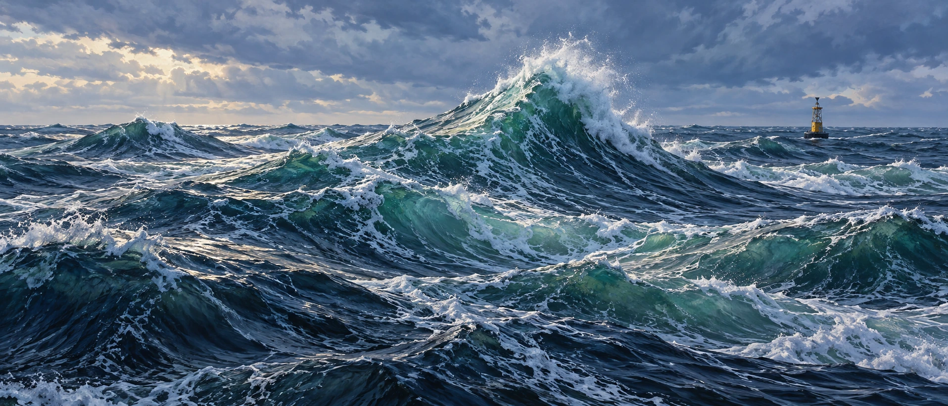
A wave can be remarkable because of its neighbors. A twenty-metre wave in one sea state and the same-height wave in another do not represent the same statistical surprise. To understand a rogue-wave claim, first establish what the surrounding sea was doing.

A panoramic marine painting places a steep crest among crossing ocean waves and a distant buoy.
An imagined steep crest in a crossing sea. The picture supplies no measured wave height, significant wave height or occurrence probability.

Researchers commonly use a wave-height threshold relative to the significant wave height of the record. Significant wave height describes the scale of the sea state; in a time-domain description it approximates the average height of the highest third of waves. It is not the height of every wave, and it is not a maximum.

The NOAA buoy-calculation explanation makes this distinction useful when reading a wave report. A rogue-wave threshold often used in research is a crest-to-trough height exceeding twice the significant wave height. Crest elevation above the mean surface is a different quantity.

Start with addition

Ordinary wave trains can reinforce or partly cancel one another. When several crests coincide, their contributions add. When a crest meets a trough, they can reduce the instantaneous displacement. NOAA’s overview describes constructive interference and focusing by currents among the mechanisms relevant to unusually large waves.

The model below isolates addition. It uses twelve sinusoidal components at one instant, each with an amplitude of one metre and a different wavelength. The sliders control phase: where each component sits in its cycle.

Twelve waves, one surface

Phase controls reveal linear addition with explicit limits; no rogue-wave probability is inferred.

Open twelve waves, one surface in its own window.

Press “Align all crests at the centre.” At that position, twelve contributions of one metre produce a twelve-metre elevation above the mean. Spread their phases again and the central sum changes, even though no individual component’s amplitude has changed.

These are invented inputs. The display does not calculate a significant wave height, crest-to-trough height or probability. Calling its large central value a measured rogue wave would import a statistical claim that the toy model has not established.

The record that made the question concrete

The Draupner platform measured an exceptional North Sea wave on January 1, 1995. The frequently reported values are about 25.6 metres crest to trough in a sea state with a significant wave height around 12 metres. The value of an instrument record is that neighboring waves and the exceptional event can be evaluated together.

A study of linear-interference models and ocean time series examines how assumptions about component waves and phase-space behavior affect extreme-wave occurrence. Its conclusions belong to the specified model and datasets. They do not establish a universal number of component waves required by every real ocean event.

Direction changes how a crest breaks

A real sea has direction. Waves can meet at different angles, interact with currents and steepen until the simple linear picture fails. That creates a second question beyond “Can the contributions add?”: what limits or reshapes the resulting crest?

In Oxford and Edinburgh experiments recreating aspects of the Draupner wave, researchers varied the angle between crossing wave groups. The resulting breaking behavior differed from that of a simpler following-sea arrangement. The laboratory result helps test a possible mechanism rather than replaying a unique recovered movie of the 1995 ocean.

That is the useful relationship between a model and an event. Measurements constrain the target. Controlled experiments explore which physical combinations can reproduce important features. Neither removes all uncertainty about what happened beyond the instrument’s field of observation.

Five quantities worth finding in a rogue-wave report
  • The event’s crest-to-trough height and, separately, its crest elevation.
  • The record’s significant wave height and the interval used to estimate it.
  • The instrument and its sampling limitations.
  • Wave direction, crossing seas and relevant currents.
  • Whether the quoted occurrence rate comes from observations or a model.

For example, a reported twenty-metre wave divided by a significant wave height of eight metres gives a ratio of 2.5. Dividing by twelve metres gives about 1.67. The arithmetic is elementary, but it changes the claim. The wave height must first be defined consistently in both cases.

The most interesting rogue-wave research keeps two ideas together. Addition can produce a striking crest without an exotic ingredient, while a dependable account of its rarity and breaking requires much more than a row of sine waves. The ocean’s ordinary ingredients can still create exceptional outcomes.

Sources and further exploration

Explore all 80 new articles · Browse the complete illustrated collection

Keep exploring at Incoprea.

Thursday, October 22, 2026

The SOFAR Channel: An Ocean Layer That Lets Sound Travel Far

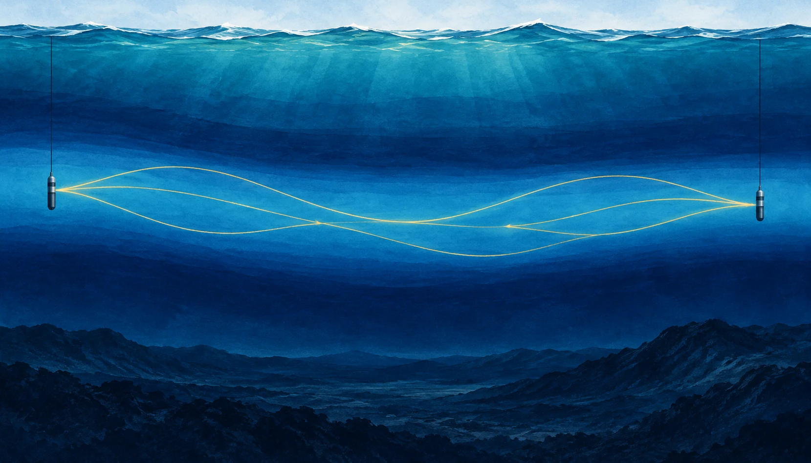
Wide ocean cutaway showing two hydrophones and gently bending gold sound paths in a blue mid-depth layer.
Conceptual illustration of a sound channel. Gold lines depict simplified ray paths, not wavelengths; scales are compressed.

A sound does not need a wall to be guided. In the open ocean, a low-frequency pulse can travel through a layer that repeatedly bends its path back toward the layer’s center. The guide is made of changing water properties. There is no pipe to find on the seabed.

The SOFAR channel—Sound Fixing and Ranging—is a reminder that the sea is not an acoustically uniform tank. Its vertical structure can matter as much as the power of the source or the sensitivity of the listener. To understand an underwater recording, you need some understanding of the water between them.

Find the slowest sound

Sound speed in seawater depends on temperature, pressure, and salinity. In a common deep-ocean profile, cooling with depth initially lowers sound speed. Farther down, increasing pressure becomes dominant and sound speed rises. Between these trends lies a minimum. NOAA’s ocean-sound explanation describes how these gradients shape the route sound takes.

Rays departing the minimum at suitable angles curve back toward it. The repeated refraction can limit losses that would occur if energy continually spread toward the surface and bottom. Low frequencies can also suffer relatively little absorption, making long-range propagation possible. The channel does not preserve every sound equally or guarantee detection at any distance.

A useful mental picture is a valley in sound speed, not a trench in the ocean floor. The axis can occur at different depths in different regions. Treat any diagram with a channel at exactly one depth as an example, not a universal ocean floor plan.

The drawing is a map of paths, not a vibrating rope

SOFAR illustrations often show a sinusoidal-looking line crossing the sea. It is easy to mistake this for the sound wave itself. Usually it represents a ray path: a simplified direction along which acoustic energy travels. The rapid pressure oscillations occur along that route; their wavelength is a separate property.

NOAA’s SOFAR guide introduces the layered-water concept. When reading the image, ask whether the horizontal and vertical scales match, whether the source sits inside the channel, and whether the drawn ray is one of several possible paths. A very flattened ocean section can make gentle bending look steep.

Those questions also explain why hearing a source does not immediately reveal its distance. A hydrophone may receive several arrivals that followed different paths. Their sequence contains information, but the loudest arrival is not necessarily the simplest geometric connection.

What made the channel important

Woods Hole Oceanographic Institution’s history and modern field account describes the long-range experiments behind the channel’s practical importance and later work on acoustic communication beneath Arctic ice. Sound can remain useful where radio and light offer limited underwater reach.

The historical experiment is best read as evidence for a physical route, not as a universal range specification. Detectability depends on frequency, source level, background noise, absorption, bathymetry, and the receiver. A successful transmission across a basin does not mean that any small speaker can communicate across the same basin.

Long-distance sound has served navigation, research, and monitoring. It also connects distant human noise sources with marine listening environments. The same physics that makes the ocean informative means a soundscape cannot always be understood by looking only at nearby traffic.

Do the travel-time arithmetic

Use a rounded sound speed of 1,500 meters per second for an idealized calculation. A 1,500-kilometer path then takes 1,000 seconds: about 16 minutes and 40 seconds. That is quick compared with a ship crossing the distance and surprisingly slow compared with an ordinary telephone conversation.

Now add a second possible path that is 15 kilometers longer. At the same rounded speed, its arrival is ten seconds later. A receiver can therefore record a sequence rather than one crisp pulse, even though both arrivals came from the same source. These are illustrative numbers, not a reconstructed ocean experiment.

The full calculation must account for how sound speed varies along each path. Temperature and currents can change the travel time too. That makes the variability both a complication for communication and a possible measurement of the water itself.

Try separating two questions in your notes: can the receiver detect the sound, and can the listener identify its source? A faint but distinctive timed signal may support a useful measurement, while a louder ambiguous sound can remain difficult to interpret. Range is only one part of a successful acoustic observation.

The Arctic does not simply copy the temperate ocean

The WHOI account describes a distinctive Arctic structure involving warm water layers of Atlantic and Pacific origin and colder intervening water. Such layering can create an acoustic duct different from the familiar deep SOFAR picture. Sea ice further changes how sound interacts with the upper boundary.

This is a useful warning against learning one attractive diagram too literally. The mechanism is refraction by a sound-speed structure; the structure must be established for the place, season, and depth of interest. A named phenomenon is a starting hypothesis about the environment, not a substitute for measuring it.

WHOI’s sound-channel animation offers another way to inspect the ray-path idea. Pause it and compare the path with the explanatory text. Ask which visible elements are actual sound recordings and which are drawn aids to understanding. The presentation combines these layers, so its caption is part of the scientific information.

A distant sound is also a sampling decision

A hydrophone placed in a channel does not produce a neutral inventory of everything that happened in the ocean. Its depth, sensitivity, frequency response, and recording schedule determine which parts of the sound field enter the archive. Long propagation can bring faraway sources within reach while leaving their geographic origin ambiguous.

A cylindrical hydrophone hanging from a cable in deep blue water
Illustrative hydrophone close-up. The instrument records pressure variations, not a view of a sound ray.

The NOAA/NPS Noise Reference Station network uses consistently calibrated recording systems so comparisons among places and times have a defensible instrumental basis. Identical equipment is not the same as identical surroundings: water depth, bathymetry, shipping, weather, and animals can differ at each site.

The team’s published account of long-term soundscape monitoring explains the purpose of establishing baseline conditions. “Baseline” here means a documented reference for comparison. It need not mean an ocean without human activity, or the quietest conditions that ever existed.

Make a listening log that could be checked later

Follow the network’s link to its creator-produced Listening to the Sea presentation. Choose one clearly captioned example. Note its location, recording interval, and whether the presentation says playback was altered. Listen once for repeated structure, then once for changes in the background. Keep your device volume fixed during the comparison.

Use three columns headed “heard,” “shown,” and “inferred.” A repeated low tone belongs in the first. A bright band at a marked frequency belongs in the second. “Passing ship” belongs in the third unless the caption or independent observation establishes the source. You can be accurate about a tone’s shape while remaining uncertain about its cause.

Now deliberately change the volume on replay. The sound becomes louder in your room, but nothing about the historical source has changed. That simple intervention exposes why an internet clip cannot, by itself, establish an absolute underwater sound level. A calibrated recording and stated processing preserve a connection that arbitrary playback gain does not.

Finally imagine the same source closer to a second receiver but outside that receiver’s favorable propagation route. Nearer need not always mean easier to detect. The sound channel matters because the ocean between source and listener is part of the instrument. A useful recording caption describes that connection rather than allowing the loudest noise to stand in for the nearest event.

A listening guide without entering the water

Use WHOI’s acoustics collection as a starting point for public recordings and explanations. Before interpreting a clip, find out whether it is raw sound, filtered sound, sped-up playback, or a sonification of non-audible measurements. A dramatic tone may be an intentional presentation choice rather than what a human diver would hear.

Then list three things you would need to infer range: the source timing or identity, a sound-speed profile, and an account of possible paths. The exercise shows how a simple recording becomes an inverse problem. The ocean has carried a message, but it has also edited the route, timing, and strength of that message on the way.

Sources and a next step

Continue exploring art, ideas, and unexpected connections at Incoprea.

LIGO’s Squeezed Light: Improving a Cosmic Measurement by Rearranging Uncertainty

LIGO listens for tiny changes in the relative lengths of long interferometer arms. Its laser light is part of the ruler. But quantum fluctuations in that light also contribute noise, limiting how clearly the instrument can measure passing gravitational waves.

One response is to prepare the light in a squeezed quantum state. The phrase sounds like a beam being physically narrowed. What is rearranged is the uncertainty associated with properties of the optical field.

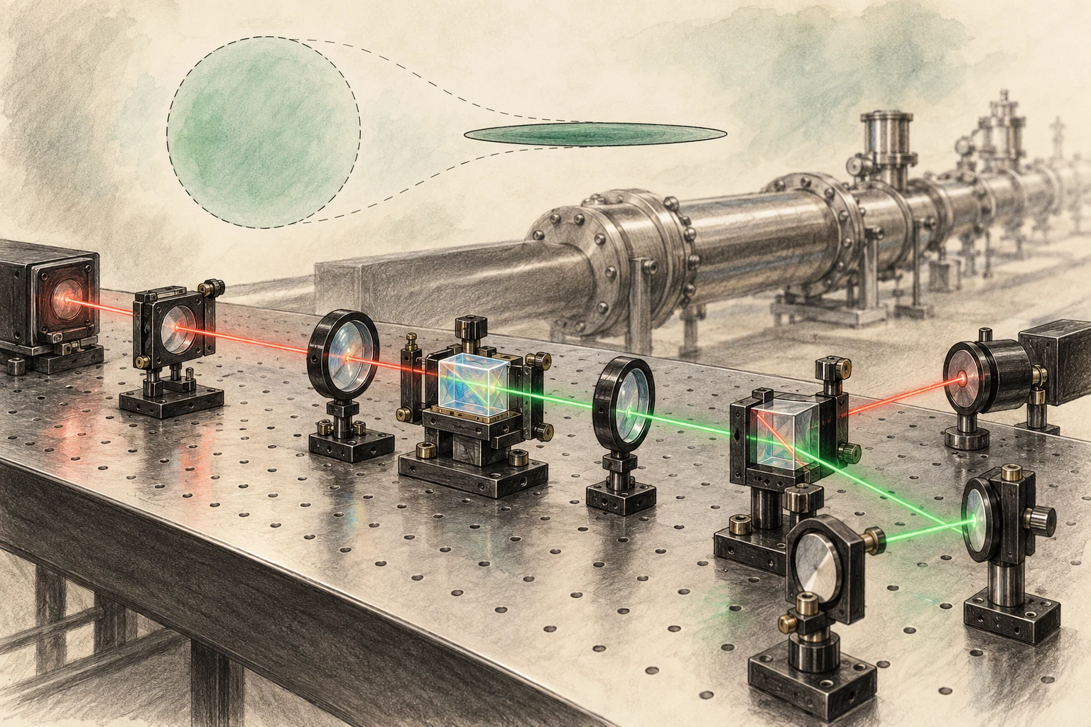
Pencil-and-watercolor optical bench with crystal, lenses, red and green paths, and a subtle circle-to-ellipse uncertainty metaphor.
Conceptual quantum-optics artwork, not a photograph or exact LIGO optical layout. The ellipse visualizes uncertainty qualitatively.

A ruler made of interference

Light traveling through the detector’s arms recombines, and changes in the relative optical paths alter the interference signal. LIGO’s sensitivity requires extraordinary control of seismic motion, thermal noise, optical losses, alignment, and many other effects.

MIT’s LIGO instrumentation overview places quantum optics within that wider engineering effort. Squeezing is one improvement in a system whose noise sources vary with frequency. Reducing one contribution does not automatically remove the others.

This frequency dependence matters because a detector does not have one universal noise number. Its sensitivity curve describes how well it measures different gravitational-wave frequencies, and different astronomical signals occupy that curve differently.

The uncertainty trade

Two field quadratures can be pictured as components analogous to amplitude and phase. Their uncertainties obey a quantum constraint. A squeezed state reduces fluctuations in one chosen combination while increasing them in another, rather than making every property simultaneously exact.

LIGO’s explainer by Lee McCuller introduces this trade through a balloon analogy. The useful part is redistribution. The analogy should not be read as a literal pressure applied to photons or a classical object hiding inside the light beam.

Draw a circle, then an ellipse with the same area. The ellipse is narrower along one direction and wider along the other. This is a conceptual picture of changed uncertainties, not a photograph of a quantum state or a complete statement of every experimental noise source.

Why squeezing one way is insufficient

At higher frequencies, photon-counting fluctuations contribute shot noise. At lower frequencies, fluctuations in radiation pressure can move the mirrors and create measurement back action. A squeezing choice that improves one part of the spectrum can worsen another.

McCuller and colleagues’ 2020 frequency-dependent-squeezing paper explains the need to rotate the squeezed quadrature with frequency. The goal is to match the uncertainty reduction to the part of the measurement that matters at each frequency.

Increasing laser power is not a universal alternative, because power affects shot noise and radiation-pressure effects differently and introduces practical thermal and optical challenges. Detector improvement is a balance of coupled limits.

A filter cavity changes the orientation

A carefully controlled optical cavity can rotate the squeezing angle in a frequency-dependent way. That lets the detector benefit across a broader band. The word “filter” refers to its optical action on the field, not a software operation that removes unwanted wiggles after a gravitational-wave event has been recorded.

MIT’s precision-measurement page describes the 300-meter filter cavities installed at the LIGO sites in 2023. The infrastructure is substantial because tiny optical losses, alignment errors, and phase noise can degrade the prepared quantum state’s benefit.

Loss is especially instructive: it mixes in ordinary vacuum fluctuations and reduces the observable squeezing. A remarkable state prepared at one point must survive the entire relevant optical path to improve the actual detector output.

What optical loss adds back

The uncertainty ellipse can be beautifully narrow at its source and less useful by the time it reaches the measurement. Loss reduces the contribution of the prepared state and mixes in ordinary vacuum fluctuations. Better preparation and better delivery are therefore linked engineering tasks.

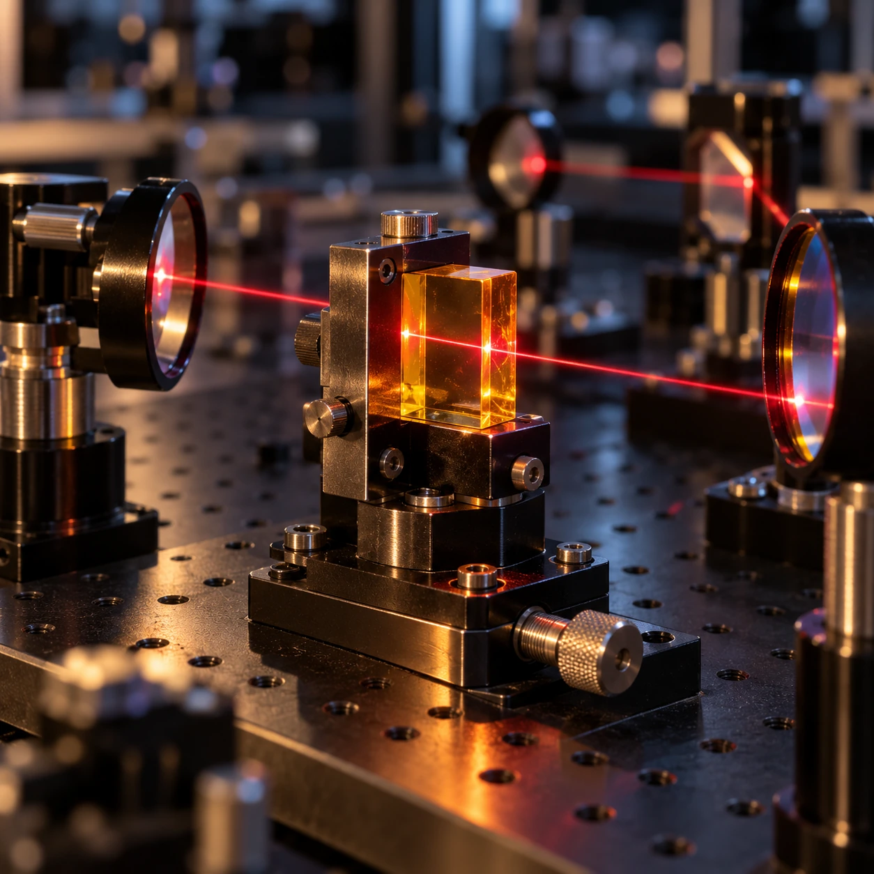
Optical crystal, mirror mounts and lenses on a dark laboratory table
Conceptual optics bench, not the exact LIGO layout. The model isolates one ideal loss relationship.

Sheila Dwyer’s LIGO thesis examines optical losses and squeezing-angle fluctuations as limits on observed quantum-noise reduction. A later LIGO squeezed-light thesis follows the sensing and control problem through detector operation and proposed improvements. These accounts have their own dates and configurations; they are evidence about the physical limitations, not a claim that one historical performance figure applies to every present observing state.

Send an invented squeezed variance through a lossy path

Normalize the ordinary vacuum variance to 1. In an ideal single-quadrature loss model, the output variance is ηV + (1−η), where V is the input variance and η is the retained fraction. If V=0.25 and η=0.8, the output is 0.4. It remains below 1, but part of the prepared reduction has been lost.

Preserve a squeezed variance

Explore ηV+(1−η), with separate variance and amplitude-noise readouts.

Open this activity in its own window.

The control below isolates this mixing relationship. At complete transmission it returns V. At complete loss it returns 1 regardless of how strongly the original state was squeezed. Those limits make the physical lesson visible without a full interferometer calculation.

Compare improving V from 0.25 to 0.1 when η is 0.95 and when η is 0.2. In the second case, the output remains much closer to ordinary vacuum. A more impressive source does not buy the same improvement when most of its useful contribution is lost.

This is variance, not amplitude. The model also reports the square root as the corresponding normalized amplitude-noise factor so the two are not confused. It omits squeezing-angle error, frequency-dependent rotation, radiation-pressure coupling, and classical noise. Its single number cannot reproduce LIGO’s sensitivity curve.

For the final reading task, look for where an experimental paper states the observed squeezing and where it describes the generated or inferred level before losses. They answer different questions. Then check whether the comparison includes a full detector noise budget or an isolated optical measurement.

The added apparatus study brings this abstract point back to materials: lenses, mirrors, alignment, and interfaces through which the state must pass. Quantum measurement does not become less practical because it is subtle. Its benefit depends on the remarkably practical work of preserving what was prepared.

The full detector is the test

The collaboration’s broadband-enhancement paper reports the realization of frequency-dependent squeezing in full-scale detectors, reducing both shot-noise and radiation-pressure contributions over the relevant band. That is a stronger result than demonstrating a narrow optical effect on a separate bench.

MIT’s 2023 account explains the instrument advance and its expected astronomical value. The projection concerns improved reach under stated conditions, not a promise that every observing period must detect a fixed number of mergers.

Actual detection counts depend on observing time, duty cycle, data quality, source populations, and chance. A sensitivity improvement creates the possibility of seeing more; the universe supplies the events.

A small reach change can mean a larger search volume

In an idealized nearby, uniform Euclidean population, increasing detection distance by 10 percent increases the enclosed volume by 1.1 cubed, or about 33 percent. That is an original geometric example, not LIGO’s measured gain from a particular upgrade.

The example explains why modest range improvements matter. Real astrophysical reach depends on source masses, orientation, waveform, detector network, cosmology at larger distances, and analysis thresholds. The simple cube is an intuition, not a replacement for an instrument’s published sensitivity calculation.

It also clarifies the difference between distance and event-rate language. A statement that a detector can survey a larger volume should not be rewritten as the same percentage increase in distance.

The detector comparison also needs a consistent operating state. A curve recorded on a quiet day at one laser power cannot be attributed entirely to squeezing if the reference came from different conditions. Controlled comparisons and a noise model help separate the quantum improvement from other changes. This is a general experimental lesson made unusually demanding by LIGO: the desired effect can be real while the size assigned to it is wrong unless the comparison isolates the relevant variable.

Read a noise curve as a budget

  1. Check the horizontal frequency axis and the vertical strain-noise units.
  2. Identify whether the curve shows amplitude or power, because improvements scale differently.
  3. Compare squeezed and unsqueezed operation over the whole band.
  4. Look for the classical-noise floor that limits the visible gain.
  5. Read whether the result is measured, modeled, or a design target.

Then revisit the circle-and-ellipse sketch. Rotate the ellipse on the page and imagine a different orientation being appropriate at different frequencies. The drawing cannot reproduce the detector’s quantum correlations, but it makes the purpose of frequency dependence easier to hold in mind.

LIGO’s squeezed light does not abolish uncertainty. It uses a deeper understanding of uncertainty to build a better ruler, turning quantum physics from a source of noise into part of the measurement strategy.

Sources and a next step

Continue exploring art, ideas, and unexpected connections at Incoprea.

Famous Last Meals is now in paperback — stories, history and 25 recipes

Famous Last Meals: Stories, History, and Recipes is now available in paperback on Amazon. The illustrated collection brings together 23 his...