
Showing posts with label Scientific Instruments. Show all posts

Thursday, October 22, 2026

Lake Baikal’s Underwater Telescope Waits for a Flash in the Dark

Conceptual cutaway showing vertical strings of optical detectors in deep blue lake water and a faint cone of blue light.
Conceptual cutaway, not a photograph or engineering drawing. Depth is compressed and sensors enlarged; real Baikal-GVD modules lie far below the surface.

A telescope usually asks you to look up. At Lake Baikal, the important direction is down: through winter ice, through hundreds of meters of water, toward suspended strings of light detectors. There is no giant lens at the bottom. The lake itself is part of the instrument.

The attraction is a particle that almost always refuses to stop. A high-energy neutrino can cross an enormous amount of matter without an encounter. On a rare occasion it interacts in or near the instrumented water, producing charged particles. Those secondaries can leave a brief optical signature. The scientific task is to turn a scatter of tiny flashes into a defensible account of an invisible visitor.

Why darkness is useful, but emptiness is not

Neutrino astronomy needs two apparently contradictory things: a great deal of material for a rare interaction to happen in, and enough transparency to see what that interaction produces. Clear deep water provides both. Instead of building a tank comparable to a substantial part of a lake, researchers distribute sensors through a natural volume.

The Baikal-GVD collaboration’s detector description places optical modules on vertical strings, with the upper modules roughly 700 meters below the surface and the lower ones near 1,240 meters. Anchors and submerged buoyancy hold the strings in position. They still move, so the array continually measures their locations acoustically. A detector cannot infer a light pulse’s journey accurately if it does not know where its receiving ends were.

Think of that as surveying a concert hall while the seats slowly drift. Timing alone is insufficient. A slightly different assumed seat position creates a different apparent travel path. Here the geometry is a calibration problem, not a decorative detail of construction.

The blue light does not break a speed limit

The flash is Cherenkov radiation. A charged particle can move through water faster than light travels in water, while remaining slower than light’s vacuum speed. IceCube’s explanation of the same detection principle makes this distinction explicit. No signal overtakes the universal vacuum limit.

An analogy is a wake: a disturbance outruns the medium’s own wave propagation and creates an organized pattern. The analogy is useful for picturing geometry, but the optical process is not literally a boat wake. Photons arrive at different sensors at different times, after traveling through water that absorbs and scatters some of them.

The instrument records light intensity and timing, then reconstruction software compares plausible events with those observations. The most appealing illustration of a glowing track is therefore the beginning of a question. What pattern of secondary particles could have produced these particular detections, and how well do competing explanations fit?

Two shapes, different information

A long muon track and a compact particle cascade leave different signatures. IceCube’s account of cascade searches explains the tradeoff: extended tracks can be especially helpful for direction, while contained cascades can provide strong information about deposited energy. Neither is a photograph of the original neutrino.

Reading an event display
What you seeWhat to ask
Spheres of different sizesDoes size represent sensor hardware or recorded light?
A sequence of colorsIs the color key showing arrival time rather than temperature?
A fitted line or coneWhich parts are reconstruction, and which are measurements?
An estimated sky directionHow large is the directional uncertainty?

This reading guide matters because event displays compress several layers of interpretation into one attractive image. A line that looks exact on a screen can carry an uncertainty region too small to notice at that scale, or one omitted from a simplified public graphic.

A worked timing intuition

Consider a deliberately simplified example. Take light’s speed in water as approximately 225 million meters per second. A straight 100-meter optical path takes about 0.44 microseconds. That is less than a millionth of a second, yet differences on that scale are meaningful when reconstructing a large detector’s pattern.

This calculation is an illustration, not a Baikal event measurement. Real reconstruction includes wavelength-dependent optical properties, scattered light, sensor response, and particle geometry. Its purpose is to show why synchronized clocks and surveyed detector positions become the telescope’s equivalent of carefully ground optics.

The hard part is deciding where the particle came from

Earth’s atmosphere also makes neutrinos when cosmic rays strike it. Cosmic-ray showers produce other particles that can create background signals. A detected candidate must therefore be tested against expected backgrounds; high energy alone is not a label saying “distant galaxy.” A source association also needs a statistically appropriate comparison with chance coincidences in direction and time.

The collaboration’s 2023 status paper describes the growing instrument and its reconstruction and physics work. Read such results with their dates attached. A detector is expanded in stages, so an old event sample and today’s array configuration are different things. This article avoids treating an advertised final volume as a constant historical property.

There is a pleasing reversal here. An instrument built to study remote astrophysical processes depends on very local knowledge: the lake’s optical clarity, the exact sensor positions, its clocks, and its changing conditions. The cosmic view becomes credible because the nearby water is understood carefully.

Try the data-display habit elsewhere

The IceCube Masterclass detection guide offers public examples of tracks, cascades, and more complex signatures. Before reading a caption, identify what the symbols encode. Then compare your interpretation with the explanation. You are not discovering a new neutrino; you are practicing the more transferable skill of separating a measurement, a visualization, and a fitted story.

A telescope is also a selection system

Imagine an instrument that recorded every small pulse without selection. Its dataset would describe a mixture of electronic noise, ordinary light backgrounds, atmospheric particles, and rare events of interest. Triggering and later analysis narrow that mixture. This makes the selection criteria part of the scientific result: a sample chosen to favor clear tracks answers a different question from one designed to retain compact cascades.

When a result is reported, look for the observation period, the event-selection definition, and the expected background. Those three details are often more informative than an impressive-looking energy number alone. They explain what population the finding belongs to and what was excluded before the final plot appeared.

Sources and a next step

Continue exploring art, ideas, and unexpected connections at Incoprea.

Seismologists Can Make a Map From the Earth’s Background Murmur

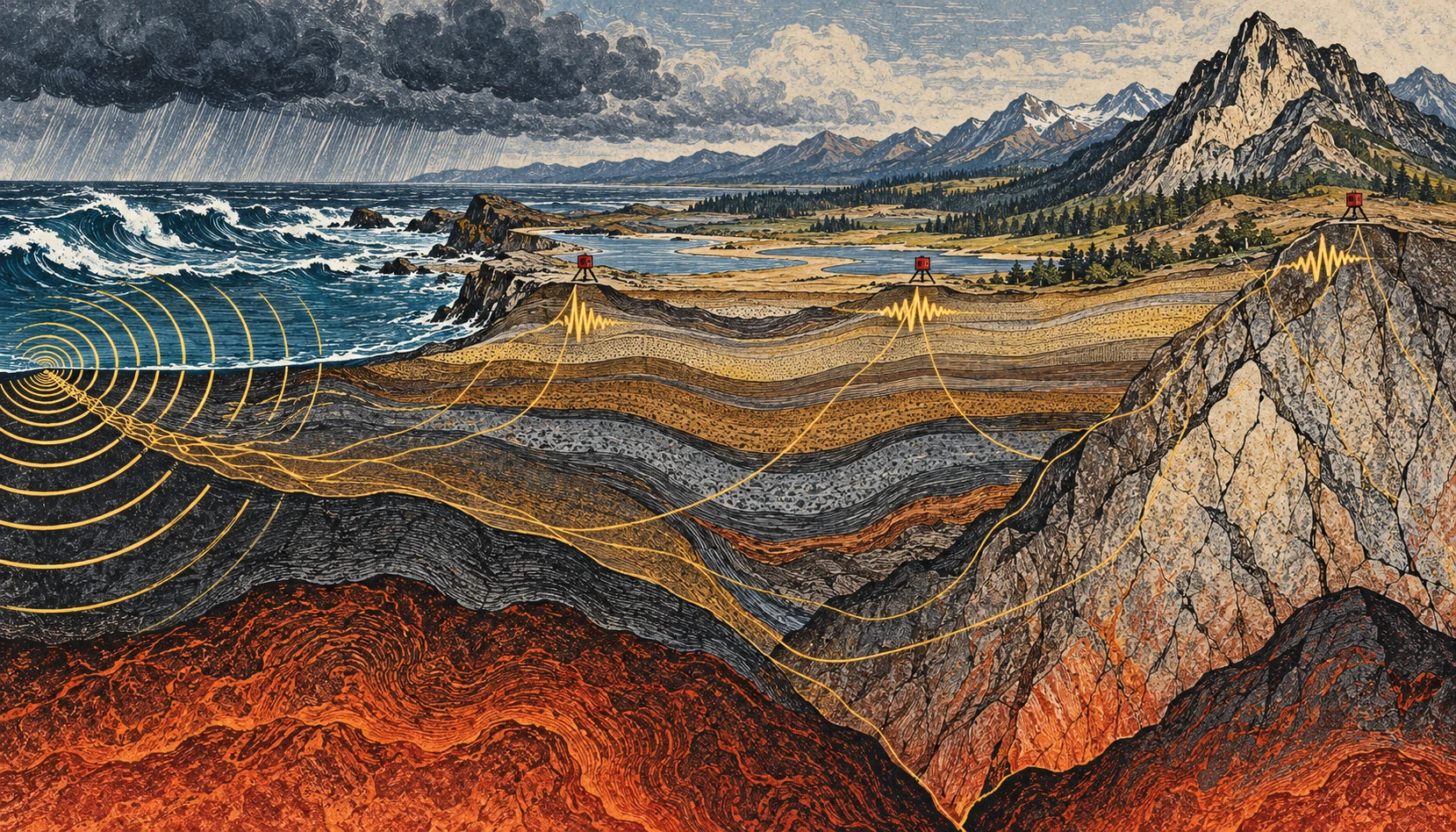
Linocut-style geological cross section from stormy coast to mountains, with small seismometers and conceptual vibration paths.
Conceptual illustration of ambient seismic noise and a sensor network; colors and paths are explanatory artwork, not tomography data.

If you could make the ground’s ordinary motion visible, a quiet day would stop looking quiet. Ocean waves, weather, traffic, and distant activity keep adding small vibrations. For an earthquake analyst these can be background. For another kind of seismology, the background is the experiment.

Ambient-noise tomography uses the continuous seismic wave field to estimate how waves travel between stations, then turns many such measurements into a model of Earth’s interior. It is a way of asking useful questions without waiting for a convenient earthquake to happen.

The ocean is part of the recording

A seismometer responds to ground motion, not merely earthquakes. USGS guidance on reading seismograms identifies background contributions from wind, human activity, and oceanic microseisms. A wiggly trace alone therefore does not establish an earthquake, much less tell you its magnitude or distance.

The ocean contribution is particularly striking. Waves interact with the solid Earth, and different mechanisms generate vibrations at different periods. The USGS account of microseisms distinguishes primary signals associated with the wave period from secondary signals associated with interactions between opposing wave components. A storm can help shake a seismometer far from the coast.

This does not mean that every visible wave drives a uniquely identifiable wiggle beneath your feet. A recording mixes many sources and propagation paths. The useful structure emerges statistically, after processing and enough observation time.

Two stations, one repeated question

Imagine two stations, A and B. Each records a long stretch of continuous motion. Shift one record relative to the other and compare them. At some time shifts, recurring wave energy is more consistently aligned than at others. Cross-correlation is the mathematical comparison that extracts this pattern.

Under suitable conditions, the correlation contains information resembling the response that would be recorded at one station if the other acted as a source. The virtual-source language is helpful, provided it is not taken literally: nobody has turned the first seismometer into a hammer. The wave field and the processing let researchers recover aspects of the path between them.

In the landmark 2005 California study by Shapiro and colleagues, a month of ambient noise from USArray stations yielded hundreds of surface-wave travel measurements. The resulting images distinguished major sedimentary basins from the faster igneous cores of mountain ranges. That is a concrete demonstration of the method, not a promise that one month is sufficient in every region.

From travel time to a map

Travel time is an integrated clue. A wave can cross several kinds of material before arriving. One measurement cannot say exactly which part of the path was slow. Many crossing paths help constrain where the slower and faster regions lie.

Picture trying to locate a traffic jam from journey times on overlapping bus routes. A slow trip might have several explanations; a whole network helps narrow them. The analogy stops at the physics, but it captures the inverse problem: infer an unseen distribution from its accumulated effect on things that passed through it.

Different surface-wave periods also respond to different depth ranges. Combining their behavior helps construct depth-dependent models. The result is a seismic-velocity model, not a literal photograph, and a velocity anomaly does not have only one possible geological cause.

A small calculation to make the ambiguity visible

Suppose two hypothetical paths are each 120 kilometers long. In a simple uniform model, a wave speed of 3 kilometers per second gives a 40-second travel time. At 2.5 kilometers per second, it takes 48 seconds. The eight-second difference is easy to see in this idealized arithmetic.

Now divide the slower route into two 60-kilometer sections. One might be fast and the other slow, yet their combined journey time could match a different, more uniform route. That is why a single average speed cannot locate a buried boundary. Additional paths and independent constraints provide the resolving power.

These are invented round numbers for understanding travel time, not measurements of California or an earthquake prediction. Real surface waves are dispersive, and researchers estimate quantities appropriate to the wave packet and method rather than applying this elementary model unmodified.

When the background changes

The noise sources do not surround a network evenly or remain constant through the seasons. That matters. USGS research on correlation amplitudes explicitly addresses how source distribution and attenuation influence the result. Reliable travel-time information does not automatically make every amplitude equally simple to interpret.

Time-lapse monitoring adds another challenge: a changed correlation can reflect a changed medium, changed noise illumination, or processing and instrument effects. Research on volcanic seismic interferometry explores how repeating measurements can track changes, but such monitoring must separate these possibilities. An interesting velocity variation alone is not a forecast with a date attached.

Listen with your eyes

Open a public seismogram through the USGS reading guide. Find the time markings and check how the trace is scaled. Before naming a wiggle, ask whether several stations recorded it, whether the timing fits a traveling event, and whether the background level changed. You are practicing observation rather than diagnosing a hazard.

The remarkable shift is intellectual as much as technical. “Noise” names a relationship between a signal and a question. Change the question, add the right network, and keep the assumptions visible, and the ground’s restless background can reveal structure that an isolated dramatic event would miss.

Resolution belongs on the map

Draw ten lines crossing a square, with most of them clustered along its left edge. You now have many paths but poor coverage of the right side. Adding a hundred nearly identical left-side lines will not solve the imbalance. A tomographic network has an analogous problem: measurement count and spatial resolving power are related, but they are not interchangeable.

This is why a convincing velocity image needs information about station geometry, path coverage, uncertainty, and recovery tests. A visually smooth color transition might be a feature of the inversion’s regularization rather than a sharp geological boundary. The appropriate question is not simply whether the map looks detailed, but which sizes and locations of structure the available observations can actually distinguish.

Sources and a next step

Continue exploring art, ideas, and unexpected connections at Incoprea.
The Atmosphere Has Tides You Can Find in a Barometer

A barometer is usually treated as a weather-change detector: pressure falls as a storm approaches, then rises behind it. But hidden within the irregular weather is a repeating signal tied to the solar day. The atmosphere has tides.

They are not simply ocean tides moved upward. Much of the atmospheric tidal response is driven by periodic solar heating. Daily patterns of absorption and heating excite global-scale waves in pressure, temperature, density, and wind.

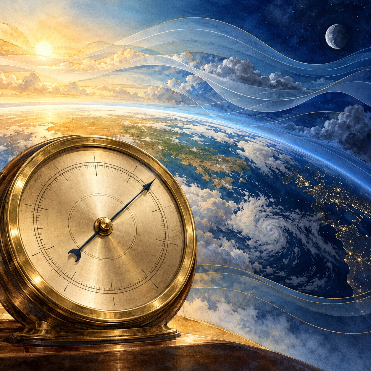
Conceptual mixed-media artwork of an unnumbered brass barometer against a curved day-night Earth and translucent atmospheric bands.
AI-generated conceptual artwork of atmospheric pressure tides. The instrument face and colored air bands are illustrative, not data.

Heating can drive a planet-sized rhythm

As Earth rotates, the solar heating pattern moves relative to the ground. Water vapor, ozone, clouds, and other processes distribute that heating through the atmosphere. The response includes components with a 24-hour period and a 12-hour period, called diurnal and semidiurnal tides.

NCAR’s Global Scale Wave Model description explains how modeled tidal forcing includes solar absorption by water vapor and ozone and how background winds, temperature, and dissipation influence the response. The atmosphere is not expanding and contracting as one simple balloon.

Gravitational atmospheric tides also exist, but they should not be confused with the dominant thermally driven components discussed here. A shared word points to a periodic planetary response, not necessarily the same forcing mechanism in air and sea.

Twice a day is not twice as much sunshine

A daily forcing can be decomposed into harmonics. Its shape need not be a perfect sine wave; the atmosphere’s own wave structure and response determine which components become important at different heights and latitudes. A semidiurnal pressure signal therefore does not require the Sun to rise twice.

NCAR’s explanation of the diurnal tide also illustrates that different heating contributions can have different phases and partly cancel. Adding two drivers is not always equivalent to simply making the same oscillation larger.

This makes a useful analogy with music: two repeating contributions can reinforce or reduce one another depending on timing. The atmosphere is not literally a musical instrument with one fixed note, but phase is a physical quantity that affects the sum.

A pressure record contains several stories

At the surface, the familiar semidiurnal pressure tide is especially recognizable in tropical averages. Weather systems, local thermal effects, and instrument behavior can obscure it in a single day’s trace. A repeated pattern becomes clearer when many days are aligned by time and averaged.

Research on thermal tides in the tropical Atlantic examines surface pressure and related wind and precipitation patterns. The scientific interest includes the spatial structure, not merely the existence of a twice-daily wobble.

A weather app may show sea-level-adjusted pressure rather than the pressure actually measured at the station. Those products answer different questions. For a local analysis, first identify the variable, sampling interval, station altitude, and any corrections instead of combining unlike numbers.

A small home-data investigation

If you already have a stable electronic barometer or a public station series, gather several weeks of regular readings. Keep the sensor at a fixed height and temperature setting as far as possible, record missing intervals, and retain the unaltered data. Do not move it between a desk and an upstairs window mid-experiment.

  1. Plot each day against local clock time to look for repeated structure.
  2. Check whether daylight-saving changes or time-zone conversions create a shift.
  3. Subtract each day’s mean as a simple exploratory step, while noting that it does not remove every weather trend.
  4. Average by hour and compare the result with the spread among days.
  5. Repeat for different subsets, rather than trusting one attractive average.

The procedure is exploratory. It does not isolate a pure migrating solar tide, and sensor temperature sensitivity or regular indoor pressure changes could imitate a daily rhythm. If the pattern disappears when you remove a few days, that is useful evidence about its robustness.

Sampling can manufacture a rhythm

Suppose a hypothetical pressure signal repeats every 12 hours. Sampling only once daily always visits nearly the same phase; sampling every 12 hours can do the same. Neither schedule adequately shows the rise and fall. More frequent sampling reveals the shape, while careful timekeeping preserves its phase.

This is an original sampling example rather than a statement about a particular station. It illustrates why a long list of observations can still fail to resolve a periodic process. Duration and sampling interval must be chosen together.

Weather-driven changes also require care. A strong multiday trend can leak into an average or spectral estimate, especially with gaps. A frequency peak is a clue to investigate, not automatic proof of the physical source you hoped to find.

Keep the daily curves as well as their average. A repeating mean can be produced by a consistent small signal or by a few large excursions that happened at similar times. Compare the median hourly pattern and the spread if your tools allow it. If they tell a different story, investigate rather than selecting the prettier curve. The point is to find a stable relationship in the observations, not to make a household instrument reproduce a textbook diagram.

The tide grows into the upper atmosphere

Atmospheric tides can propagate upward and influence winds in the thin upper atmosphere. Their amplitudes and phases evolve as density, background flow, and dissipation change. NASA-supported work combining satellite observations and modeling investigates the migrating diurnal tide across the mesosphere and lower thermosphere.

NASA’s ICON findings connect upper-atmospheric winds and tides with electric fields in the ionosphere. Lower-atmosphere processes can thus influence a region commonly associated only with space weather.

The connection does not mean that one household pressure fluctuation predicts a satellite disturbance. It reveals a shared, vertically coupled atmosphere whose processes span scales far beyond the instrument on your table.

A barometer’s gentle repeat can be easy to overlook beside a storm’s dramatic plunge. Averaging patiently changes the view. The apparently noisy record begins to carry a regular planetary rhythm, made by sunlight and motion rather than by a visible tide line on a shore.

Sources and a next step

Continue exploring art, ideas, and unexpected connections at Incoprea.
Stellar Occultations: Measuring a Distant World by Watching a Star Disappear

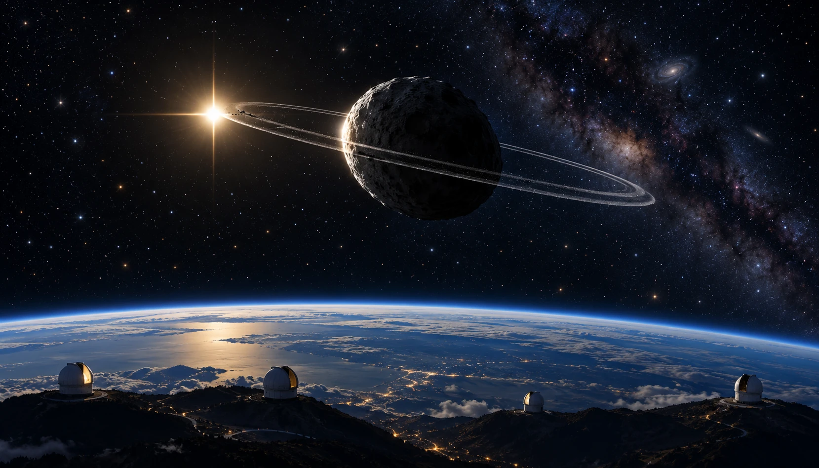
Conceptual wide illustration of a small ringed icy body occulting a distant star, with telescope sites along Earth’s curved edge.
AI-generated occultation concept, not a direct image of Chariklo. Object sizes, star separation, and telescope spacing are exaggerated.

A star disappears for a few seconds. To most viewers, that sounds like a failed observation. To an occultation team, the timing of the darkness can be the measurement they planned for months.

When a Solar System body crosses the line of sight to a distant star, it casts a moving shadow across the observer’s location. Measuring the star’s changing brightness can reveal the foreground object’s size, shape, atmosphere, or rings at a level of detail difficult to obtain from a direct image.

The star supplies the backlight

The distant star acts approximately as a small light source, while the nearer body and any surrounding material block or refract some of its light. The observation becomes a light curve: brightness measured repeatedly through the event.

An airless solid edge can produce a relatively abrupt disappearance. A tenuous atmosphere can alter the light more gradually through refraction and extinction. Rings can produce additional dips before and after the main body’s passage. The actual curve also includes finite exposure time, diffraction, the star’s apparent size, and instrument behavior.

ESO’s account of Chariklo’s ring discovery shows how unexpected secondary dips led to a striking result. Telescopes at several sites watched the 2013 event, allowing the pattern to be tested across different paths through the shadow.

One site measures a chord

A telescope’s disappearance and reappearance times define a path across the object’s projected silhouette when combined with the shadow’s velocity. This path is called a chord. A short chord can pass near an edge; it need not imply that the whole body is small.

Several stations provide several chords. Together they constrain the silhouette more strongly than one site can. A station with no occultation can also be useful, setting a limit on where the shadow did not pass, provided its timing and sensitivity are adequate.

Imagine drawing a circle and laying three parallel strings across it. Each string has a different length, though all belong to the same circle. Now replace the circle with an ellipse. The exercise makes clear why one duration is insufficient to establish a unique shape.

A simple duration calculation

Suppose a hypothetical shadow moves at 20 kilometers per second and a solid-body occultation lasts 8 seconds. Ignoring other complications, the corresponding chord length is 160 kilometers. If the observing cadence is one frame per second, the timing resolution becomes a substantial fraction of the event.

These invented numbers do not describe Chariklo’s actual measurements. They show why accurate clocks and rapid photometry matter. A tenth of a second at that speed corresponds to 2 kilometers of chord distance before including other uncertainties.

For narrow rings, finite exposure can smear a dip. A shallow feature may be genuinely low opacity, partly unresolved, diluted by background light, or affected by other observational factors. The model has to account for the instrument as well as the object.

The ring announcement was not a direct close-up

The Chariklo discovery paper presents the multi-chord evidence for two narrow rings. The ring geometry emerged from light losses and their timing, not from a spacecraft visiting the object and photographing the particles.

That distinction is easy to lose when an artist’s impression accompanies a news story. The impression helps readers picture the inferred system. The measured light curves and geometric fit are the evidence.

ESO’s observation video offers a useful next step: watch the actual stellar brightness change before looking again at the polished ring illustration. The small dip becomes more impressive when you know what information it carries.

Webb changed the observing location

A space telescope follows its own trajectory, so predicting an occultation requires the star position, the foreground object’s orbit, and the observatory’s location. A ground-based shadow track alone is not enough.

NASA’s 2023 Chariklo report describes Webb observations and explicitly labels the report as science in progress at the time. That qualification belongs with the original announcement rather than being silently removed in retelling.

The more general lesson is that precise astrometry—the measurement of positions—makes the dramatic event possible. The eventual few-second curve rests on years of orbit and star-position work, scheduling, and accurate timekeeping.

Changing opacity has more than one interpretation

Santos-Sanz and colleagues’ subsequent analysis of the Webb occultation reports an inner-ring signature stronger than in earlier observations and a weaker near-infrared signature for the outer ring. The authors discuss temporal change and wavelength-dependent opacity as possibilities that are not mutually exclusive.

A weaker dip in a different wavelength does not automatically mean that a ring lost the same fraction of its mass. Particle size, composition, viewing geometry, and optical properties affect the relation between brightness loss and material. New observations at matched wavelengths can help separate those explanations.

This is where the subject moves beyond a simple discovery story. A ring system can be well established while its origin, stability, and evolving particle population remain active research questions.

Try adding a timing uncertainty to the hypothetical eight-second event. If each edge is uncertain, the chord length should carry uncertainty too, and an uncertain shadow velocity adds another contribution. The resulting silhouette is a fitted region rather than an infinitely thin outline. This does not diminish the method’s precision; it explains what precision means. A reader can then compare two inferred shapes without pretending that either was measured with a physical ruler placed beside the object.

Read a light curve in three passes

  1. First identify the baseline, noise, and any comparison-star correction.
  2. Then mark the main disappearance and additional dips without deciding what they mean.
  3. Finally compare the model, observing cadence, and other stations’ chords.

Keep a distinction between an observed feature and the object inferred to explain it. An isolated dip might be instrumental; matching features across independent sites offer stronger evidence. A model that explains timing, geometry, and repeated observations is more persuasive than a resemblance in one curve.

Occultations turn absence into a ruler. The star’s brief disappearance is useful because the darkness has a location, a duration, and a carefully measured context.

Sources and a next step

Continue exploring art, ideas, and unexpected connections at Incoprea.
LIGO’s Squeezed Light: Improving a Cosmic Measurement by Rearranging Uncertainty

LIGO listens for tiny changes in the relative lengths of long interferometer arms. Its laser light is part of the ruler. But quantum fluctuations in that light also contribute noise, limiting how clearly the instrument can measure passing gravitational waves.

One response is to prepare the light in a squeezed quantum state. The phrase sounds like a beam being physically narrowed. What is rearranged is the uncertainty associated with properties of the optical field.

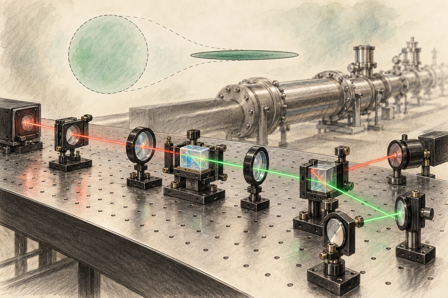
Pencil-and-watercolor optical bench with crystal, lenses, red and green paths, and a subtle circle-to-ellipse uncertainty metaphor.
AI-generated conceptual quantum-optics artwork, not a photograph or exact LIGO optical layout. The ellipse visualizes uncertainty qualitatively.

A ruler made of interference

Light traveling through the detector’s arms recombines, and changes in the relative optical paths alter the interference signal. LIGO’s sensitivity requires extraordinary control of seismic motion, thermal noise, optical losses, alignment, and many other effects.

MIT’s LIGO instrumentation overview places quantum optics within that wider engineering effort. Squeezing is one improvement in a system whose noise sources vary with frequency. Reducing one contribution does not automatically remove the others.

This frequency dependence matters because a detector does not have one universal noise number. Its sensitivity curve describes how well it measures different gravitational-wave frequencies, and different astronomical signals occupy that curve differently.

The uncertainty trade

Two field quadratures can be pictured as components analogous to amplitude and phase. Their uncertainties obey a quantum constraint. A squeezed state reduces fluctuations in one chosen combination while increasing them in another, rather than making every property simultaneously exact.

LIGO’s explainer by Lee McCuller introduces this trade through a balloon analogy. The useful part is redistribution. The analogy should not be read as a literal pressure applied to photons or a classical object hiding inside the light beam.

Draw a circle, then an ellipse with the same area. The ellipse is narrower along one direction and wider along the other. This is a conceptual picture of changed uncertainties, not a photograph of a quantum state or a complete statement of every experimental noise source.

Why squeezing one way is insufficient

At higher frequencies, photon-counting fluctuations contribute shot noise. At lower frequencies, fluctuations in radiation pressure can move the mirrors and create measurement back action. A squeezing choice that improves one part of the spectrum can worsen another.

McCuller and colleagues’ 2020 frequency-dependent-squeezing paper explains the need to rotate the squeezed quadrature with frequency. The goal is to match the uncertainty reduction to the part of the measurement that matters at each frequency.

Increasing laser power is not a universal alternative, because power affects shot noise and radiation-pressure effects differently and introduces practical thermal and optical challenges. Detector improvement is a balance of coupled limits.

A filter cavity changes the orientation

A carefully controlled optical cavity can rotate the squeezing angle in a frequency-dependent way. That lets the detector benefit across a broader band. The word “filter” refers to its optical action on the field, not a software operation that removes unwanted wiggles after a gravitational-wave event has been recorded.

MIT’s precision-measurement page describes the 300-meter filter cavities installed at the LIGO sites in 2023. The infrastructure is substantial because tiny optical losses, alignment errors, and phase noise can degrade the prepared quantum state’s benefit.

Loss is especially instructive: it mixes in ordinary vacuum fluctuations and reduces the observable squeezing. A remarkable state prepared at one point must survive the entire relevant optical path to improve the actual detector output.

The full detector is the test

The collaboration’s broadband-enhancement paper reports the realization of frequency-dependent squeezing in full-scale detectors, reducing both shot-noise and radiation-pressure contributions over the relevant band. That is a stronger result than demonstrating a narrow optical effect on a separate bench.

MIT’s 2023 account explains the instrument advance and its expected astronomical value. The projection concerns improved reach under stated conditions, not a promise that every observing period must detect a fixed number of mergers.

Actual detection counts depend on observing time, duty cycle, data quality, source populations, and chance. A sensitivity improvement creates the possibility of seeing more; the universe supplies the events.

A small reach change can mean a larger search volume

In an idealized nearby, uniform Euclidean population, increasing detection distance by 10 percent increases the enclosed volume by 1.1 cubed, or about 33 percent. That is an original geometric example, not LIGO’s measured gain from a particular upgrade.

The example explains why modest range improvements matter. Real astrophysical reach depends on source masses, orientation, waveform, detector network, cosmology at larger distances, and analysis thresholds. The simple cube is an intuition, not a replacement for an instrument’s published sensitivity calculation.

It also clarifies the difference between distance and event-rate language. A statement that a detector can survey a larger volume should not be rewritten as the same percentage increase in distance.

The detector comparison also needs a consistent operating state. A curve recorded on a quiet day at one laser power cannot be attributed entirely to squeezing if the reference came from different conditions. Controlled comparisons and a noise model help separate the quantum improvement from other changes. This is a general experimental lesson made unusually demanding by LIGO: the desired effect can be real while the size assigned to it is wrong unless the comparison isolates the relevant variable.

Read a noise curve as a budget

  1. Check the horizontal frequency axis and the vertical strain-noise units.
  2. Identify whether the curve shows amplitude or power, because improvements scale differently.
  3. Compare squeezed and unsqueezed operation over the whole band.
  4. Look for the classical-noise floor that limits the visible gain.
  5. Read whether the result is measured, modeled, or a design target.

Then revisit the circle-and-ellipse sketch. Rotate the ellipse on the page and imagine a different orientation being appropriate at different frequencies. The drawing cannot reproduce the detector’s quantum correlations, but it makes the purpose of frequency dependence easier to hold in mind.

LIGO’s squeezed light does not abolish uncertainty. It uses a deeper understanding of uncertainty to build a better ruler, turning quantum physics from a source of noise into part of the measurement strategy.

Sources and a next step

Continue exploring art, ideas, and unexpected connections at Incoprea.
The Elevator With Three Working Buttons

Case 50 · shortest-path challenge · Hard · About 10-15 minutes The archive elevator has a peculiar test mode. Its floor display works, but o...