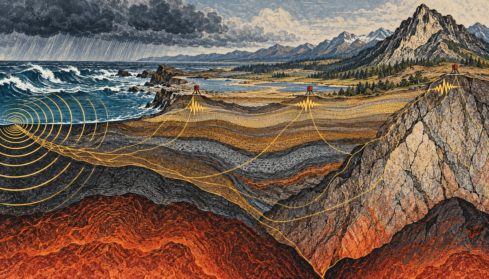
If you could make the ground’s ordinary motion visible, a quiet day would stop looking quiet. Ocean waves, weather, traffic, and distant activity keep adding small vibrations. For an earthquake analyst these can be background. For another kind of seismology, the background is the experiment.
Ambient-noise tomography uses the continuous seismic wave field to estimate how waves travel between stations, then turns many such measurements into a model of Earth’s interior. It is a way of asking useful questions without waiting for a convenient earthquake to happen.
The ocean is part of the recording
A seismometer responds to ground motion, not merely earthquakes. USGS guidance on reading seismograms identifies background contributions from wind, human activity, and oceanic microseisms. A wiggly trace alone therefore does not establish an earthquake, much less tell you its magnitude or distance.
The ocean contribution is particularly striking. Waves interact with the solid Earth, and different mechanisms generate vibrations at different periods. The USGS account of microseisms distinguishes primary signals associated with the wave period from secondary signals associated with interactions between opposing wave components. A storm can help shake a seismometer far from the coast.
This does not mean that every visible wave drives a uniquely identifiable wiggle beneath your feet. A recording mixes many sources and propagation paths. The useful structure emerges statistically, after processing and enough observation time.
Two stations, one repeated question
Imagine two stations, A and B. Each records a long stretch of continuous motion. Shift one record relative to the other and compare them. At some time shifts, recurring wave energy is more consistently aligned than at others. Cross-correlation is the mathematical comparison that extracts this pattern.
Under suitable conditions, the correlation contains information resembling the response that would be recorded at one station if the other acted as a source. The virtual-source language is helpful, provided it is not taken literally: nobody has turned the first seismometer into a hammer. The wave field and the processing let researchers recover aspects of the path between them.
In the landmark 2005 California study by Shapiro and colleagues, a month of ambient noise from USArray stations yielded hundreds of surface-wave travel measurements. The resulting images distinguished major sedimentary basins from the faster igneous cores of mountain ranges. That is a concrete demonstration of the method, not a promise that one month is sufficient in every region.
From travel time to a map
Travel time is an integrated clue. A wave can cross several kinds of material before arriving. One measurement cannot say exactly which part of the path was slow. Many crossing paths help constrain where the slower and faster regions lie.
Picture trying to locate a traffic jam from journey times on overlapping bus routes. A slow trip might have several explanations; a whole network helps narrow them. The analogy stops at the physics, but it captures the inverse problem: infer an unseen distribution from its accumulated effect on things that passed through it.
Different surface-wave periods also respond to different depth ranges. Combining their behavior helps construct depth-dependent models. The result is a seismic-velocity model, not a literal photograph, and a velocity anomaly does not have only one possible geological cause.
A small calculation to make the ambiguity visible
Suppose two hypothetical paths are each 120 kilometers long. In a simple uniform model, a wave speed of 3 kilometers per second gives a 40-second travel time. At 2.5 kilometers per second, it takes 48 seconds. The eight-second difference is easy to see in this idealized arithmetic.
Now divide the slower route into two 60-kilometer sections. One might be fast and the other slow, yet their combined journey time could match a different, more uniform route. That is why a single average speed cannot locate a buried boundary. Additional paths and independent constraints provide the resolving power.
These are invented round numbers for understanding travel time, not measurements of California or an earthquake prediction. Real surface waves are dispersive, and researchers estimate quantities appropriate to the wave packet and method rather than applying this elementary model unmodified.
When the background changes
The noise sources do not surround a network evenly or remain constant through the seasons. That matters. USGS research on correlation amplitudes explicitly addresses how source distribution and attenuation influence the result. Reliable travel-time information does not automatically make every amplitude equally simple to interpret.
Time-lapse monitoring adds another challenge: a changed correlation can reflect a changed medium, changed noise illumination, or processing and instrument effects. Research on volcanic seismic interferometry explores how repeating measurements can track changes, but such monitoring must separate these possibilities. An interesting velocity variation alone is not a forecast with a date attached.
Listen with your eyes
Open a public seismogram through the USGS reading guide. Find the time markings and check how the trace is scaled. Before naming a wiggle, ask whether several stations recorded it, whether the timing fits a traveling event, and whether the background level changed. You are practicing observation rather than diagnosing a hazard.
The remarkable shift is intellectual as much as technical. “Noise” names a relationship between a signal and a question. Change the question, add the right network, and keep the assumptions visible, and the ground’s restless background can reveal structure that an isolated dramatic event would miss.
Resolution belongs on the map
Draw ten lines crossing a square, with most of them clustered along its left edge. You now have many paths but poor coverage of the right side. Adding a hundred nearly identical left-side lines will not solve the imbalance. A tomographic network has an analogous problem: measurement count and spatial resolving power are related, but they are not interchangeable.
This is why a convincing velocity image needs information about station geometry, path coverage, uncertainty, and recovery tests. A visually smooth color transition might be a feature of the inversion’s regularization rather than a sharp geological boundary. The appropriate question is not simply whether the map looks detailed, but which sizes and locations of structure the available observations can actually distinguish.
Sources and a next step
- USGS: about seismograms and their background
- Aster and colleagues: microseism mechanisms
- Shapiro and colleagues: 2005 ambient-noise tomography
- USGS: correlation amplitudes and noise sources
- USGS: monitoring volcanic systems with interferometry
Continue exploring art, ideas, and unexpected connections at Incoprea.