Showing posts with label Weather. Show all posts

Thursday, October 22, 2026

An Atmospheric River Is a Moving Water Budget, Not a River in the Sky

An atmospheric river is easiest to misunderstand when its name is taken literally. It is not a raised channel of liquid water crossing the sky. It is an elongated region of strong water-vapor transport: moist air moving fast enough, through enough of the atmospheric column, to shift a substantial water budget.

That wording matters for anyone looking at a forecast. A bright moisture plume is not the same thing as rain already falling, and the largest instantaneous transport is not the only feature that determines the result at a particular watershed.

Conceptual panorama of a translucent moisture plume crossing the Pacific toward coastal mountains with rain and high-elevation snow.
Conceptual moisture-transport illustration, not a satellite observation or storm forecast. The visible plume represents invisible vapor transport.

Moisture multiplied by motion

NOAA’s introduction describes the long, narrow transport regions that play an important role in moving water vapor outside the tropics. When moist air is lifted, including over mountains, cooling can produce precipitation. The amount and location depend on the weather system and terrain.

The diagnostic quantity often shown is integrated vapor transport, or IVT. It combines water-vapor content with horizontal wind through a vertical atmospheric column. Its common unit is kilograms per meter per second: transport through a vertical curtain of unit width.

That unit is different from millimeters of rain. Turning transport into rainfall requires knowing how much moisture converges, rises, condenses, falls, and remains in or leaves the region. A large through-flow can pass over a location without all of it being deposited there.

Make the units concrete

Take a hypothetical IVT of 500 kilograms per meter per second across a 100-kilometer-wide curtain perpendicular to the flow. Multiplying by 100,000 meters gives 50 million kilograms per second. At 1,000 kilograms per cubic meter of liquid water, that is a water-equivalent volume transport of 50,000 cubic meters per second.

This is an idealized unit conversion, not a measurement of a named storm and not the flow of a sky-borne liquid river. It says how much water vapor crosses the selected curtain in the example. The curtain’s orientation matters: transport oblique to it needs the perpendicular component.

Now hold the transport steady for 12 hours, then imagine the same value lasting 48 hours. Four times the time means four times the cumulative transport across that curtain. Even before adding land conditions, duration changes the scale of the event.

A scale that includes time

The 2019 atmospheric-river scale developed by Ralph and colleagues combines peak IVT with duration at a location. Its categories are intended to communicate a spectrum from beneficial to increasingly hazardous conditions rather than treating every atmospheric river as a disaster.

Scripps’ explanation of the scale describes the role of the 24-to 48-hour duration range and the adjustments for shorter or longer events. A scale category is still not a complete flood forecast. It describes a transport event, while the watershed has its own recent history and vulnerabilities.

A dry catchment and a saturated one can respond differently to similar precipitation. Snow level can shift the balance between immediate runoff and stored snow. Recently burned terrain, steep slopes, drainage capacity, and reservoir operations can also change local outcomes.

Read the plume, then read the spread

CW 3 E’s forecast guide explains its plume diagrams and ensemble products. Thin lines represent different model members, helping expose uncertainty in timing, strength, and duration. A single thick forecast line is easier to look at, but can conceal a meaningful spread among plausible evolutions.

Use a forecast as a set of questions. When does transport begin? How long does it stay elevated? Do model members agree on the peak? Does the plume aim at the same stretch of coast in successive forecasts? A small landfall shift can place strong flow against a different mountain barrier or watershed.

The page also notes that its analysis representation of IVT is modeled rather than a direct continuous measurement everywhere. That distinction should travel with a screenshot. A colored map can be an analysis, a forecast, or a composite; the label determines how it should be read.

A watershed comparison

Same transport label, different setting
SettingAdditional question
Dry basin after a long rain-free periodHow much storage is available in soils and reservoirs?
Already wet basinHow quickly will new rainfall become runoff?
Mountain catchmentWhere is the snow level and how does terrain face the flow?
Recently burned slopeWhat local debris-flow guidance has been issued?

The table is an interpretation aid, not site-specific hazard advice. For an actual event, local weather and emergency guidance supply the necessary place-based information.

Here is a second scale check: if a hypothetical ten millimeters of rain falls uniformly over a hundred square kilometers, the water volume is one million cubic meters. The amount reaching a channel immediately can be much smaller or arrive later, depending on storage and routing. Comparing this rainfall-volume calculation with the earlier transport calculation shows why they are different budgets. One crosses an atmospheric curtain; the other is deposited over a land area. Keeping their units visible prevents an impressive vapor-flow number from being mistaken for an inevitable flood volume.

Why researchers fly into the uncertainty

Atmospheric River Reconnaissance targets observations over the otherwise sparsely sampled ocean. Aircraft dropsondes measure vertical profiles; added observations can improve the starting state of forecast models and help researchers investigate which regions most affect later predictions.

The point is more subtle than “more data is always better.” Measurements must be placed, timed, quality-controlled, and assimilated so that they reduce the uncertainties relevant to the forecast. Sensitivity analysis helps identify where an observation can be especially informative.

After reading an event summary, try making a two-line account: one line for the atmosphere’s transport and one for the land’s response. Add the uncertainty to each. This keeps a useful scientific term from becoming a dramatic synonym for rain, and helps you see why the same atmospheric process can replenish a region’s water supply in one episode and overwhelm it in another.

How would you know the flight helped?

A research aircraft can bring back a beautiful profile and still leave a harder question unanswered: did those measurements improve the forecast people ultimately used? Testing that requires a comparison. Researchers can run a forecasting system with a selected observation set and run a matched experiment withholding those observations.
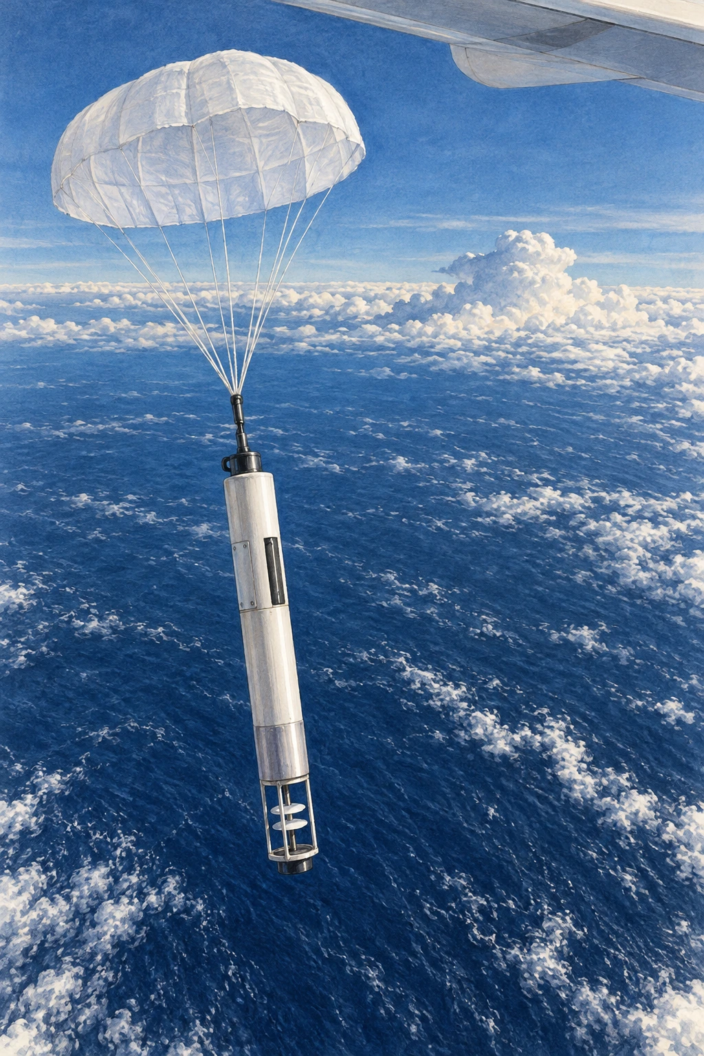
A parachute-supported research dropsonde descending over the Pacific
Illustrative research dropsonde; it is not a record of a particular flight.

A study of the 2020 AR observing campaign compared a control including reconnaissance dropsondes with a denial experiment excluding them in a specified global forecasting system. That design asks about the contribution of those data within that system and period. It does not show that aircraft are the only useful observations or that every individual flight must improve every local prediction.

A later sampling-strategy study summarized by its CW3E authors explored mission frequency and sonde spacing during a six-day 2021 sequence. Reducing temporal or spatial sampling degraded skill in the experiments reported there. The placement and repetition of observations were part of the result, not interchangeable details of flight logistics.

Design a fair forecast comparison

Use a fictional example with two forecast runs for the same storm. Run A places a heavy-rain band 100 kilometers too far north. Run B puts it 20 kilometers too far north but predicts an excessive peak amount. Which is better? You cannot answer fully until you state what is being scored.

Make three rows: location of the band, total rainfall over the watershed, and maximum point rainfall. Give each a separate assessment. A model can improve on one metric while worsening on another. One screenshot with a convincing storm shape cannot settle all three.

Next require the runs to use the same model version, forecast start time, and verification observations. Otherwise an apparent benefit might come from a different upgrade or a more favorable comparison window. Finally compare several lead times rather than selecting the one with the largest improvement.

The exercise explains why field campaigns and forecast evaluation belong together. Measuring the atmosphere improves the starting evidence. Demonstrating a useful forecast benefit needs a second experiment that follows those measurements through assimilation, prediction, and verification. The dropsonde’s descent is only the beginning of its scientific journey.

Sources and a next step

Continue exploring art, ideas, and unexpected connections at Incoprea.

The Nocturnal Low-Level Jet: A Fast River of Air Above a Quiet Night

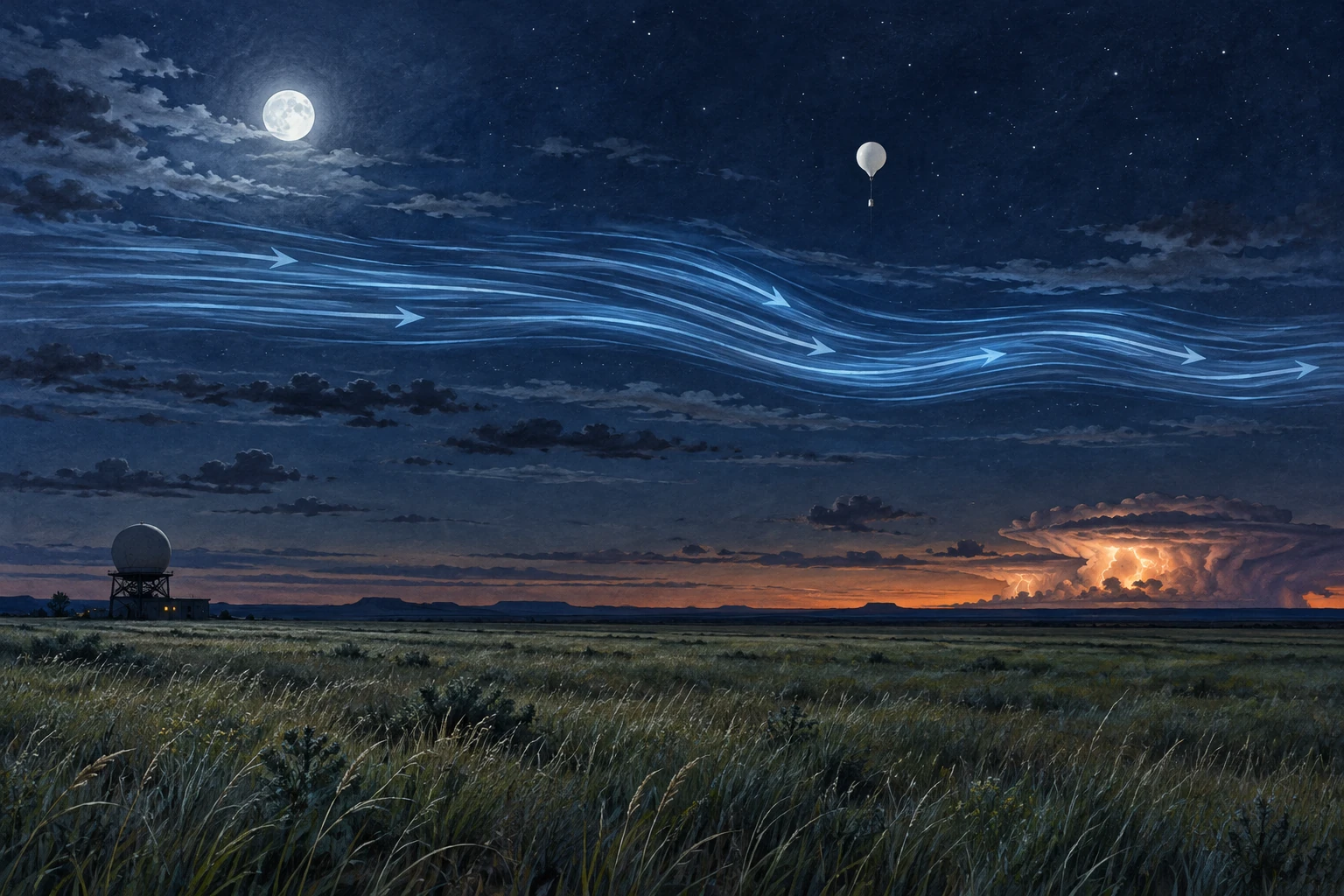
Moonlit Plains landscape with a conceptual blue airflow band above quiet grass, a weather balloon, and distant storm.
Conceptual illustration of a nocturnal low-level jet. Airflow streaks are visual aids, not visible air or measurements of a specific night.

The grass can be almost still while a fast stream of air moves a few hundred meters overhead. On a warm-season night in the Great Plains, the strongest low-level wind may be above the cooled surface layer rather than at your face.

The nocturnal low-level jet is important partly because of that separation. It can transport moisture and momentum through a night that feels quiet on the ground, helping shape the environment in which thunderstorms develop and persist.

Sunset changes the coupling

During daylight, turbulent mixing connects a deeper atmospheric layer with the surface. After sunset, surface cooling can produce a stable layer that reduces this vertical exchange. Winds above the most strongly cooled layer become less constrained by surface friction, and their adjustment can produce a wind-speed maximum.

The rotating Earth matters too. The wind’s adjustment includes an inertial oscillation, while regional pressure gradients, terrain slopes, and large-scale weather provide additional influences. There is no single switch that turns every low-level jet on at sunset.

The National Weather Service glossary identifies the common warm-season nocturnal southerly wind maximum over the Plains. Its training discussion also distinguishes nocturnal jets from low-level maxima associated with midlatitude cyclones. The same short label can cover mechanisms that overlap but are not identical.

Low does not mean surface

A jet is a maximum within a vertical wind profile. To establish one, observations must show how speed changes with height, including above the maximum. A strong wind reported at one level does not by itself reveal the full shape.

Picture two profiles. In the first, speed rises steadily from the ground to the top of the chart. In the second, it rises, reaches a peak, then declines. Only the second sketch demonstrates a local low-level maximum within the observed layer. The first might still contain one higher up, but the available profile has not shown it.

This is why a surface anemometer and an upper-air sounding answer different questions. Their disagreement can be a real atmospheric structure rather than a faulty instrument.

The night storms that prompted a field campaign

The 2015 PECAN campaign—Plains Elevated Convection at Night—focused on warm-season precipitation over the southern Great Plains. Its research setting included a stable boundary layer, a nocturnal low-level jet, and instability located above that stable layer.

That combination challenges the simple expectation that thunderstorms must be fed by warm air rising directly from a hot afternoon surface. Elevated inflow can supply storms after the ground layer cools. The jet helps move moisture, but storm initiation and maintenance also depend on lift, instability, boundaries, and existing storm systems.

Correlation between a stronger jet and an intense nocturnal convective system does not make jet speed a complete storm forecast. The physical setting has several ingredients, and their arrangement in space and time matters.

What the instruments add

PECAN’s instrument overview describes a combination of mobile and fixed profiling systems, radars, lidars, soundings, and aircraft. These methods were chosen to observe both the winds and the thermodynamic structure that ordinary surface observations could miss.

A wind profiler helps identify the jet’s height and evolution. Temperature and humidity profiles reveal the stable surface layer and potential elevated instability. Radar follows precipitation and storm organization. Combining them makes a causal account more testable than looking at a dramatic radar image alone.

Measurements also sample different volumes. A balloon drifts, a radar scans, and an aircraft traverses a path. A good analysis accounts for those sampling differences rather than assuming all instruments saw the same parcel at the same instant.

Try a moisture-transport thought experiment

Imagine a current of air carrying the same water-vapor concentration on two nights. If it moves twice as fast through the same cross-sectional area for the same duration, its idealized vapor transport doubles. Now imagine the faster current is much drier: the final transport need not double at all.

This is why wind alone is not the water budget. Moisture content, depth, direction, and duration belong in the account. The example deliberately leaves out convergence, condensation, and changing geometry; it illustrates one part of transport rather than predicting precipitation.

Next rotate the flow so that it runs along a storm boundary instead of crossing it. The same speed can feed a system differently. Direction and the location of the receiving weather feature are as important as the number on a wind-speed scale.

For a simple profile test, put a ten-meter-per-second wind at the surface, a twenty-meter-per-second wind above it, and a fifteen-meter-per-second wind higher still. You have drawn a maximum. Now remove the highest observation. The remaining data show increasing speed but no confirmed peak. The atmosphere has not changed; the evidence available to describe it has. This small example explains why incomplete soundings deserve a different conclusion from complete profiles.

A reading guide for a nighttime wind plot

  1. Check whether height is above ground or above sea level.
  2. Find the speed maximum and confirm observations extend above it.
  3. Compare direction as well as speed through the profile.
  4. Read temperature and humidity alongside the wind.
  5. Look at several times, because the jet evolves during the night.

For a real severe-weather situation, use official forecasts and warnings. This guide is for understanding archived or educational profiles, not for making a personal flight or storm-chasing decision.

A storm can send a wave ahead of itself

The jet is one part of a nighttime setting that can also support traveling disturbances. A thunderstorm’s outflow can encounter a stable lower layer and generate an atmospheric bore: a propagating adjustment of the layered air that may be followed by waves. The resulting lift can matter even where rain has not yet arrived.

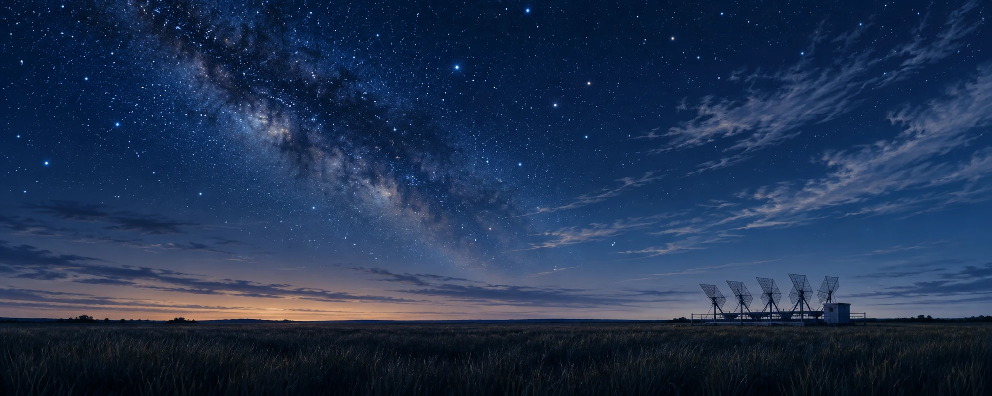
A research wind profiler beside dark Great Plains grass under a broad night sky
Quiet-ground observational scene; the instrument’s returns would reveal the air aloft.

The PECAN research overview included storm-generated wave-like disturbances among its objectives. The team’s operations plan treated bores as a specific observational target. The distinction matters: a nocturnal wind maximum and a moving bore are different features that can interact within the same environment.

Think of a layered atmosphere as having a structure that can be displaced, rather than a uniform block merely pushed across the ground. A bore can move a change through that structure while individual air parcels follow more complicated paths. The familiar wave-versus-material distinction reappears, now with implications for where elevated air may be lifted.

Three instruments, three arrival times

Imagine a fictional research site. At midnight a pressure sensor records a small step. Several minutes later a profiling instrument shows the stable layer displaced upward. Rain begins half an hour after that. These observations could motivate a bore hypothesis, but the sequence alone does not prove it. Other boundaries and local effects can alter pressure and profiles.

On paper, place the site between two additional observing stations. What would a propagating feature predict? You would expect a spatially ordered timing pattern rather than three unrelated local changes. Add a radar cross section or repeated thermodynamic profiles and specify what additional structure would strengthen the explanation.

Now move only the rain-start time. The disturbance’s apparent speed should be estimated from the observations tracking the disturbance, not from a later precipitation edge that may have a different motion. This is a small but consequential choice about what feature is actually being followed.

The activity is an interpretation of invented evidence, not a storm warning procedure. Its value is to make a quiet night less deceptively simple. A surface can cool, a jet can transport air above it, and a traveling adjustment can change the lift supplied to that air. The scientific account becomes stronger when those roles are measured separately before they are combined.

A long history of asking where the maximum is

Bonner’s 1968 low-level-jet climatology illustrates how the subject became a systematic question about frequency, geography, height, and time of day. Modern observing networks add detail, but the basic discipline remains: define the feature, sample its profile, and compare many cases.

The nocturnal jet changes how a quiet evening should be imagined. Calm at the surface is a local observation. Above it, the atmosphere can be busy transporting the ingredients of tomorrow’s rainfall.

Sources and a next step

Continue exploring art, ideas, and unexpected connections at Incoprea.
Wednesday, October 14, 2026

How an Erupting Volcano Builds Its Own Lightning Storm

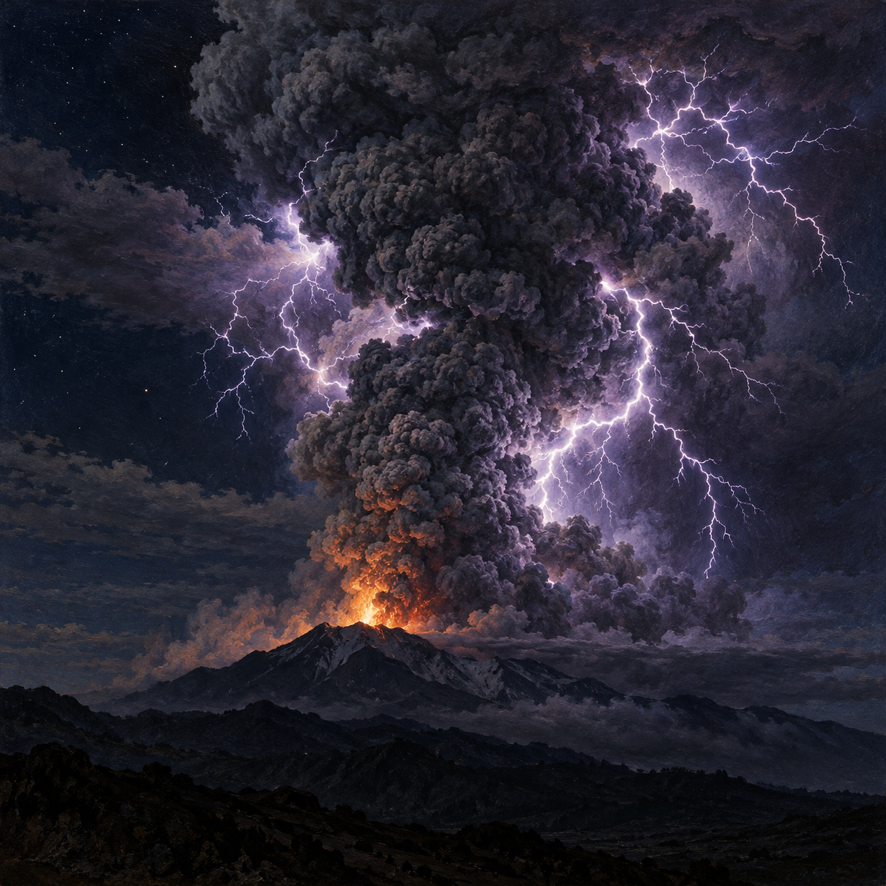
Illustration of branching lightning illuminating the ash plume above an erupting volcano at night.
An imagined eruption shows lightning within a volcanic ash plume.

A volcanic plume is already a startling sight: a mountain sends fragmented rock and gas into the sky. Then lightning branches through the ash, turning the eruption into something that appears to belong to a fantasy painting. Yet the flashes are ordinary electricity produced under extraordinary conditions.

Volcanic lightning reveals that an ash plume is much more than a cloud of dirty smoke. It is a moving mixture of particles, gas, water and sometimes ice. As those ingredients interact, they can separate electric charge strongly enough for a discharge.

Ash can become electrically active

Near the vent, rock breaks apart and particles collide. Fragmentation and particle interactions can contribute to electrical charging. Farther up, rising motion and differences among particles help redistribute charge through the plume.

Once an electric field becomes strong enough, a conducting path forms through the air and a lightning discharge occurs. The process can operate in several parts of an eruption, from the region immediately above the vent to the high spreading cloud.

It is therefore misleading to give every volcanic flash one universal recipe. A low, ash-rich jet and a towering wet plume need not build charge in exactly the same way. The importance of different mechanisms varies with eruption conditions.

Charge separation needs a moving mixture

A collection of charged particles is not automatically a lightning storm. Charges also have to become separated in a way that builds a sufficiently strong electric field. An erupting plume supplies motion across many scales: fragmentation near the source, particle collisions, upward transport and the sorting of material as the cloud develops.

Think of the difference between mixing two colors thoroughly and carrying them to opposite ends of a container. Having both colors present does not create the same large-scale arrangement. The analogy is only about separation; electric charge is governed by its own interactions and the surrounding air's ability to insulate or conduct.

As the field grows, a discharge provides a path through which charge can move. The visible flash is the brief result of a developing electrical system. Its branches do not trace every ash particle or display a complete map of the plume's contents. Much of the relevant process occurs before the camera records the bright line.

A volcano can borrow a thunderstorm's machinery

Ice becomes especially important in some tall plumes. Water carried upward can coexist with ice in a cold, turbulent region, allowing collisions similar to those that electrify meteorological thunderstorms.

USGS researchers studying Alaska's Bogoslof eruptions in 2016–2017 found detectable lightning in some explosive events and none in others. In the analyzed examples, flashes appeared after plumes rose above the atmospheric freezing level. Modeling supported ice-related charging as an important part of the explanation.

The January 2022 Hunga eruption in Tonga offered an exceptionally energetic example. Seawater blasted into the plume supplied abundant moisture. Researchers linked its tremendous electrical activity to interactions among volcanic ash, supercooled water and hailstones, recording more than 192,000 lightning flashes over the event they studied.

Read the time series alongside the spectacular image

The Bogoslof investigation is instructive because some explosive events produced detectable lightning and others did not. In its sample, 32 of 70 events did. The researchers combined lightning observations with satellite images, photographs, sound and plume models. That comparison let them ask what changed before the electrical activity began, instead of assuming that every eruption had to flash.

Try organizing the observations into a sequence: eruption onset, plume rise, entry into colder air, detected flashes. A delayed onset carries information that a photograph of one flash cannot. The association with ice-forming conditions supported a thunderstorm-style contribution in those studied plumes while allowing ash collisions nearer the vent to have a role too.

The Hunga numbers also benefit from a careful distinction. The 2023 study described just over 192,000 flashes made up of nearly 500,000 electrical pulses. A flash and a pulse are different counting units. Mixing them produces impressive but incompatible totals. The peak rate likewise refers to a particular interval, rather than the average throughout an eruption.

Before comparing two volcanic lightning records, ask what the sensors counted and which region they could detect. Optical and radio measurements do not simply duplicate one another; combining them can reveal timing and location that one source alone misses. A reported absence may reflect genuinely weak activity, an unsuitable charging environment or limits of observation. This is why electrical detection can be a powerful monitoring clue while remaining part of a larger evidence system.

The flashes carry information

Lightning is not merely decoration around an eruption. Radio and optical sensors can detect electrical activity from far away, helping scientists identify explosive activity and follow changes in a plume. That is particularly valuable at remote volcanoes where direct observation is difficult.

But the absence of detected lightning does not prove an absence of ash. Bogoslof's non-lightning explosive events make that limitation clear. Electrical observations work best alongside satellites, seismic records and other monitoring tools.

Sources and further reading: USGS: Volcanic ash and lightning · USGS: Ice charging during the Bogoslof eruption · USGS: Lightning during the Hunga eruption

Famous Last Meals is now in paperback — stories, history and 25 recipes

Famous Last Meals: Stories, History, and Recipes is now available in paperback on Amazon. The illustrated collection brings together 23 his...