Showing posts with label Mathematics. Show all posts

Sunday, October 25, 2026

A Planimeter Measures an Area by Walking Its Edge

Put a tracing point on the edge of an irregular lake drawn on a map. Follow the shoreline until you arrive back where you began. A small mechanical wheel has turned during the trip, and its reading can tell you the lake's area.

The instrument is a planimeter. Its achievement is more surprising than measuring how far the point travelled. The useful result concerns the space inside the boundary, even though the tracing point never has to visit every patch of that interior.

Illustration of a two-arm polar planimeter resting over an irregular closed outline.
A polar planimeter turns a trip around a boundary into an area reading through the motion of a small wheel.

Find the fixed point, then the moving one

A polar planimeter commonly has two arms joined at an elbow. A weighted pole fixes one end in place on the drawing surface. A tracer at the other end follows the outline. The joint allows the arms to change their angle as the tracer moves.

A small measuring wheel responds selectively to that motion. It rolls readily in one direction and can slide sideways in another. Its axis is arranged along the tracer arm, so its rolling direction is perpendicular to that arm.

Consequently, the wheel does not simply register the distance travelled by the tracer. Different parts of the boundary contribute differently, according to the instrument's position and direction of movement. The net reading accumulates these contributions over a complete trip.

Royal Museums Greenwich's polar planimeter includes a weighted pole, a magnifying glass and a calibration checking bar. Those accessories make the purpose tangible. This was an instrument for making and checking measurements, with scales that had to be set and read.

How a boundary can account for an interior

Think first about a shape divided into adjacent little regions. A boundary shared by two neighbours is traversed in opposite directions when each region is walked around consistently. In a signed accumulation, those internal contributions cancel. Only the outside boundary remains.

That cancellation is a useful intuition for Green's theorem, which connects an appropriately defined accumulation around a closed curve with a quantity over its enclosed region. The planimeter's geometry makes a boundary accumulation correspond to area.

Oliver Knill's mathematical explanation at Harvard develops that connection explicitly. You do not need to perform the calculus to see why a closed trip matters. The instrument must finish the boundary account; stopping halfway leaves an incomplete result.

The signed nature of the measurement also matters. Reversing the direction of tracing reverses the sign of the ideal net accumulation. The physical area stays positive; the direction and instrument convention tell the operator how to interpret the reading.

Choose between distance and area

Try this paper puzzle. Draw a square 4 centimetres on each side. Next draw a rectangle 1 centimetre wide and 7 centimetres long. Both boundaries have the same total length: 16 centimetres. Imagine carefully tracing each with a correctly calibrated planimeter.

Should the two readings be equal because the tracing point travels the same distance? Decide before opening the comparison.

Compare the results

The square encloses 16 square centimetres; the rectangle encloses 7. An ideal area measurement distinguishes them despite their equal perimeters. A wheel that merely counted the tracer's total travelling distance would fail this test. The planimeter's selective rolling and changing geometry make the distinction possible.

Now give the square a small inward notch. Following the notch increases the distance traced while reducing enclosed area. That single alteration makes the difference between the two kinds of measurement especially clear.

On a real instrument, a narrow notch may also be harder to trace accurately. The mathematical distinction survives, while the practical difficulty reminds us that the operator's hand contributes uncertainty.

Read the map's scale twice

Suppose a traced region occupies 3 square centimetres on a map whose scale is 1:10,000. One centimetre represents 100 metres. A square centimetre therefore represents a square measuring 100 metres on each side: 10,000 square metres.

The region represents 30,000 square metres, or 3 hectares. Applying the linear scale only once would produce the wrong kind of quantity. Area requires scaling in two directions.

Two different conversions
On this mapOn the ground
1 centimetre of length100 metres of length
1 square centimetre of area10,000 square metres of area
3 square centimetres of area30,000 square metres, or 3 hectares

This calculation assumes the stated map scale applies appropriately to the region. A planimeter measures the drawing placed beneath it. It cannot repair a distorted reproduction or decide whether a thick shoreline should be followed along its inner edge, outer edge or centre.

A good reading begins before tracing

Inspect the Smithsonian's collection of polar planimeters and compare the weighted pole, arm adjustment and scale arrangements. Look for what would stay fixed and what would move. The photographs offer a usable object study without depending on old browser applets.

For an actual measurement, the outline has to be within the instrument's reach. The setup and calibration must suit the model and pole position. A broad loop enclosing the pole can require a different correction from an ordinary pole-outside measurement; the instrument's own instructions determine the procedure.

Repeating a trace tests consistency, while checking a known area tests calibration. Those are different questions. A person can repeat the same wrong setting very neatly.

The planimeter is a compact example of mathematics embodied in a mechanism. The weighted pole limits motion, the arms organise it, and the wheel adds selected parts together. By the time the tracer returns home, a trip around the edge has become an account of the space within.


Sources and further reading

Explore more art, stories and discoveries at Incoprea.

Saturday, October 24, 2026

One Tile Can Fill a Plane Without Giving It a Repeating Grid

A tabletop covered in repeated shapes seems to invite a repeating plan. Slide the pattern far enough, and surely the same arrangement should line up again. An aperiodic monotile challenges that expectation: one tile shape can cover the infinite plane while its geometry rules out every periodic tiling.

Orange and turquoise polygon paper pieces form an irregular patch on a dark tabletop.
Conceptual paper tiles introduce the search for structure. These shapes are not the mathematically certified hat; use the creators’ linked tools for its actual geometry.

The distinction is subtle and worth exploring slowly. The shape repeats, local clusters recur, and larger organization can still exist. What is absent is a nonzero translation that carries the entire infinite tiling exactly onto itself. Repetition of an ingredient is not the same thing as a repeating global grid.

First distinguish a choice from a constraint

You can arrange ordinary square tiles in colored patterns that never settle into a repeating color sequence. That does not make a plain square an aperiodic tile. The square also admits the familiar periodic grid. A shape that permits a nonperiodic arrangement has not necessarily forced aperiodicity.

In Smith, Myers, Kaplan, and Goodman-Strauss's hat paper, the authors prove that a particular polygon can tile the plane but cannot do so periodically. They establish larger clusters and hierarchical structure, rather than treating a visually irregular sample as a proof about infinity.

The illustration above uses conceptual paper pieces. They are not the certified hat geometry and should not be used to test its mathematical claim. The exact shapes, substitution tools, and proof resources are available on the creators' project page.

A small patch cannot display an infinite guarantee

Imagine a photograph of a very large floor whose repeating unit is wider than the photograph. Inside the frame, you might fail to find a repeat even though one exists elsewhere. Conversely, a local cluster can recur inside an aperiodic tiling without producing a translation that works everywhere.

This gives you a better question for an image: what exactly repeats, and how far does the evidence reach? A single tile, a cluster of several tiles, and the entire arrangement are different objects of comparison.

Visit the creators' interactive application through their project page. Begin with a small displayed patch. Choose a recognizable cluster and look for another occurrence, allowing rotation if you are studying local similarity. Then ask whether the same displacement carries every surrounding tile into agreement. Finding one matching cluster answers the first question, not the second.

The larger pieces have their own organization

The hat research constructs metatiles—clusters that can be treated as larger building blocks—and substitution rules. That hierarchical viewpoint links local fitting to the structure of arbitrarily large regions. An apparently irregular field can contain strong organization without possessing a repeating translational unit.

For a paper exercise, draw a box around one cluster in a screenshot from the creators' tool. Describe the cluster using position and orientation, not only color. Now imagine making the observation window larger. Which apparent matches survive when their neighborhoods are included? You are testing the scope of a local claim, while leaving the infinite theorem to the proof.

Color is especially tempting. The project images use color to help reveal arrangements, but the hat result concerns geometry without extra colored matching rules. If you mentally recolor a tile, you have not changed the polygon that fits against its neighbors.

Turning a tile over changes the question

The later chiral-monotile paper makes an important distinction explicit: every tiling admitted by the original hat mixes reflected and unreflected copies. The follow-up develops Spectre shapes whose geometry supports aperiodicity without requiring mirror-image copies in the same way.

Use a paper letter such as an asymmetric block shape to think about reflection. Rotating it on the table preserves its handedness. Flipping it over reverses that handedness. The operations are different even when a casual phrase such as “move the tile around” seems to include both.

A three-column pattern notebook

Record an observation, its scope, and the evidence needed to go further. For example: “this cluster appears twice”; “within this finite patch”; “does not establish a global period.” Then record the theorem separately: “the hat admits plane tilings but no periodic ones”; “all complete tilings”; “supported by the published proof.” Keeping the columns distinct makes close looking more valuable.

Finally, compare two kinds of order. A wallpaper repeat tells you how to continue by copying a fixed translational unit. A hierarchical aperiodic construction tells you how local pieces belong inside larger structures. Both can be highly organized. Only one needs a repeating grid.

The pleasure of the monotile is that a modest-looking outline can carry a demand extending far beyond any tabletop. Its edges do more than meet the next piece. Through the constraints they impose, they help determine what the whole plane can never become.

Sources and further exploration: Smith and colleagues: an aperiodic monotile; Creators: hat tools and exact geometry; Smith and colleagues: a chiral aperiodic monotile.

Explore all 50 new articles · Browse the complete illustrated collection

Explore more art, ideas, and independent projects at Incoprea.

The Extra Seat That Makes One Group Smaller

There are ten seats around the table. Three groups must share them in proportion to their size. You work out a rule, check the arithmetic and distribute every seat. Then somebody brings an eleventh chair. Surely no group can be worse off.

Under the largest-remainder method, one can. The surprise is called the Alabama paradox. It is not a story about a population shrinking, a vote being removed or an accountant losing a chair. The population weights stay fixed while the total allocation grows.

Small wooden chairs are divided among three colored trays, with an additional chair outside.
Adding a unit changes every quota and the contest among fractional remainders. The trays are a metaphor, not the counted example.

Build the smallest useful scene

Use three fictional groups with weights 6, 6 and 2. Their total is 14. With ten seats, their exact proportional quotas are 60/14, 60/14 and 20/14: approximately 4.286, 4.286 and 1.429.

The rule first gives everyone the whole-number part: four seats, four seats and one seat. Nine seats have been assigned. The final seat goes to the largest fractional remainder. Group C’s remainder is 6/14; A and B each have 4/14. C receives the last seat, so the final distribution is 4, 4, 2.

This is the Hamilton, or largest-remainder, approach described in the Census Bureau’s methods account. The numbers here are an original compact illustration, not historic census populations.

Now add the chair

For eleven seats the quotas become 66/14, 66/14 and 22/14: about 4.714, 4.714 and 1.571. The whole-number allocations are again four, four and one. But two seats remain. A and B each have a remainder of 10/14, ahead of C’s 8/14. They receive those seats.

The new distribution is 5, 5, 1. C’s exact quota increased from about 1.429 to about 1.571, yet its actual seat count fell from two to one. Everyone’s quota grew; the ordering of the remainders changed. No arithmetic error is required.

You can audit this result without decimals. At ten seats, compare integer remainders 4, 4 and 6 over the common denominator 14. At eleven, compare 10, 10 and 8. The ordering has genuinely changed. Rounding a displayed quota to three decimal places cannot be blamed for the lost chair.

Add one seat; watch the remainders

A largest-remainder allocation for weights 6,6,2 shows the Alabama paradox between ten and eleven seats.

Open add one seat; watch the remainders in its own window.

Use the control to move from ten to eleven, then from eleven to twelve. Watch the fractional parts rather than only the quotas. A remainder climbs until its quota crosses an integer, where the remainder resets. The competition is continually reorganized by those crossings.

A fair-looking rule can miss a different kind of fairness

Largest remainder has an immediately attractive feature: each group receives either the floor or the ceiling of its exact quota. Our C receives its ceiling at ten seats and its floor at eleven. Both allocations respect that quota condition.

The condition that nobody should lose when the total grows is different. It is usually called house monotonicity. The Census Bureau’s historical perspective identifies the Alabama paradox as a difficulty of the Hamilton/Vinton method. The name marks an episode in apportionment history; the mechanism applies more generally wherever whole units are shared proportionally by this rule.

Distinguishing criteria is more useful than declaring the calculation “unfair” and stopping. Would your group rather preserve each exact quota’s neighboring integers, prevent losses when the pool grows, or minimize some measure of population per seat? Those are different questions. A rule should be judged against the properties it was actually chosen to deliver.

Try allocating something besides seats

Imagine three departments sharing ten identical display panels in proportion to request weights 6, 6 and 2. Write the 4–4–2 allocation. Then announce that eleven panels are available and recompute the same rule. The department with two panels now receives one.

If the panels have already been installed, that rule creates a practical problem. You might instead decide that additional panels can only be assigned, never taken back. That is a change to the allocation procedure. State it before using the rule, because a sequence of additions need not match a fresh largest-remainder allocation of the final total.

Svante Janson and Svante Linusson’s research on the paradox studies its probability under specified assumptions. The existence of such research should not be mistaken for a single universal frequency. Real populations, the chosen total and the model of changing house size all matter.

The eleventh chair has exposed a seam between continuous shares and discrete objects. Fractions can all rise smoothly. Chairs must land somewhere, one at a time. Before trusting a proportional rule, it helps to ask what happens when the table gets a little bigger.

Sources and further exploration: Census Bureau: methods of apportionment; Census Bureau: historical perspective; Janson and Linusson: probability of the Alabama paradox.

Explore all 50 new articles · Browse the complete illustrated collection

Explore more art, ideas, and independent projects at Incoprea.

Three Sensible Voters Can Make a Circle

Three friends have one free afternoon. Ada wants a garden before a concert, and a concert before a café. Ben puts the concert first, the café second and the garden last. Cora prefers the café, then the garden, then the concert.

Nobody is wavering. Nobody has an internally circular ranking. Yet if they decide by asking the group to choose between every pair, the group can chase itself around a circle.

Three people point to illustrated activity cards on a meeting table.
The cards set the scene; the exact rankings and counted majorities appear in the text and interactive ledger.

Give the options short names: A for garden, B for concert and C for café. The rankings are A–B–C, B–C–A and C–A–B. Higher on a list means preferred. Write them in three columns before continuing; the puzzle is easier to trust when your own finger can count the votes.

Follow the majority one step at a time

Ada and Cora prefer A to B, so the garden defeats the concert two votes to one. Ada and Ben prefer B to C, so the concert defeats the café. Ben and Cora prefer C to A, so the café defeats the garden. The group comparison reads A over B, B over C, C over A.

This is the Condorcet cycle. Eric Pacuit’s voting-theory lecture introduces pairwise criteria and the problem of choosing when comparisons do not supply an unambiguous winner. An option that defeats every other option in such contests is a Condorcet winner. Our three-option profile has none.

The word “majority” can disguise a changing membership. The two people supporting the first comparison are not the two supporting the second. Treating “the majority” as a single person with a stable set of desires is what makes the result seem impossible.

Let three rankings meet

Choose three complete rankings and compare pairwise majorities before following a sequential agenda.

Open let three rankings meet in its own window.

The order of questions becomes powerful

Suppose the friends use a knockout sequence. First compare the garden with the concert; let the winner face the café. A defeats B, then C defeats A. The café wins. Compare B with C first instead: B wins, then A defeats B. The garden wins. Compare C with A first and the final choice becomes the concert.

Every one of those procedures uses sincere votes and the same underlying preferences. The agenda alone changes the result. This is an original worked example of a general vulnerability, not evidence that real voters always follow a cycle or that every procedure is equally vulnerable.

Try a small intervention in the model: change Cora’s ranking from C–A–B to A–C–B. A now defeats both rivals. Her first choice changed, but her relative judgment of the other two remained consistent. The circle was a property of the whole profile, not a defect located in one person.

A result about rules, not a verdict on people

Kenneth Arrow’s Nobel lecture situates majority cycles within the larger challenge of constructing a social ordering from individual ones. Arrow’s theorem concerns a specific set of conditions on an aggregation rule. It is much broader than this example, and it does not say that every election is chaotic or that collective decisions are pointless.

The distinction between a preference and a factual prediction matters too. “I prefer the café” is not a testable assertion that the café will be open. A method that aggregates tastes is doing a different job from a method that combines uncertain observations about a fact. A majority cycle does not by itself tell you how accurate a crowd’s measurement would be.

Eric Maskin’s discussion of Arrow’s contributions helps separate reasonable requirements that may conflict. Choosing a rule means deciding which properties matter for the task, rather than searching for a magic slogan that resolves every possible profile.

Turn this into a fairer afternoon discussion

Before voting, agree on the procedure and what happens if a cycle appears. The friends might discuss intensity, practical constraints or a mixed itinerary, provided they understand that those additions change the decision problem. A garden-and-café plan is a fourth option; it should not silently be treated as one of the original three.

For a group exercise, ask everyone to rank three harmless activities privately. Count all three pairwise contests. If a winner exists, record that. If a cycle appears, display it before applying the agreed tie-breaking procedure. Do not infer anyone’s second choice from their first choice alone.

A circular group preference is a good reason to make the rules visible. The friends remain sensible people. Their combined rankings simply contain less of a single collective mind than the phrase “what the group wants” suggests.

Sources and further exploration: Eric Pacuit: voting theory lecture; Kenneth Arrow: Nobel lecture; Eric Maskin: Arrow’s contributions to social choice.

Explore all 50 new articles · Browse the complete illustrated collection

Explore more art, ideas, and independent projects at Incoprea.

Friday, October 23, 2026

The Wolf Interval Hides in a Tuning System’s Unpaid Remainder

Suppose you tune one note, then tune another a perfectly pure fifth above it. Keep going. After twelve fifths you expect to return to a familiar note name, seven octaves higher. The arithmetic disagrees. The journey overshoots, leaving a small remainder that cannot be wished away by careful workmanship.

A tuning tool and a blank notebook lie beside a wooden keyboard.
A fixed keyboard asks a limited set of pitches to serve many relationships. The arithmetic model below exposes one compromise.

This is a design problem disguised as a mistake. A fixed keyboard asks a finite set of keys to serve many harmonic relationships. Some desirable frequency ratios refuse to fit together exactly. A tuning system decides where that disagreement will be heard.

Do the journey with ratios

In John Baez's mathematical account, a pure fifth has frequency ratio 3:2 and an octave 2:1. Twelve fifths multiply frequency by (3/2)12; seven octaves multiply it by 27. Their quotient is 531441/524288, approximately 1.01364. This discrepancy is the Pythagorean comma.

The two routes end about 1.36 percent apart in frequency. That percentage is calculated from the ratio, not measured in a performance here. Musical intervals are more conveniently compared logarithmically in cents: 1,200 cents make an octave. The same remainder is about 23.46 cents.

You can verify the issue with a calculator. Multiply 1.5 by itself twelve times and compare the result with 128. Now ask a different question: how much must each of twelve identical steps be adjusted if their combined journey is to close? The answer concerns a repeating ratio, so simply subtracting a fixed frequency from every note is the wrong operation.

A wolf is tied to a particular compromise

The Lehman College physics notes compare open, closed unequal, and equal temperaments. In a twelve-note Pythagorean arrangement, preserving eleven pure fifths leaves a substantially narrowed closing interval. It is often called a wolf fifth. Other temperaments can produce a different wolf with a different size and direction of error.

Keep that last distinction. The famous wide wolf in quarter-comma meantone is not numerically the same interval as the narrowed Pythagorean closure demonstrated below. “Wolf” is a family resemblance in the problem a listener encounters, not one universal frequency ratio.

Move the closing interval

A silent ratio calculator compares a Pythagorean closing link with equal-tempered fifths. No measured instrument data.

Open move the closing interval in its own window.

The model uses twelve abstract links in a closed chain. It compares eleven pure fifths plus one closing remainder with twelve equal-tempered fifths. It deliberately avoids a historical keyboard's spelling and octave-placement conventions. Moving the marked closure changes its location in the chain, not the amount of arithmetic left over.

Give the remainder an address

Imagine programming a small musical instrument for only one piece. If the piece never crosses a particular harmonic relationship, putting the largest mismatch there might be a practical choice. Now lend the instrument to someone playing in distant keys. The hidden compromise may become the first thing they notice.

Move the closing link in the model. Choose three neighboring links as your imaginary piece's territory. Can you place the special interval outside that territory? Expand the territory to all twelve. You can no longer keep one exceptional link out of every possible journey. The exercise turns an abstract comma into a question about intended use.

Equal does not mean all ratios are pure

Equal temperament makes each semitone the same ratio, 21/12. Its seven-semitone fifth is 700 cents, slightly narrower than the pure fifth's approximately 701.96 cents. The mismatch is spread instead of collected in a single closure. This removes the exceptional fifth within this ideal twelve-note model, while giving up pure 3:2 fifths.

The Tune Smithy creator's listening notes distinguish the Pythagorean example from the original meantone use of the term. Its examples can extend the arithmetic into listening, but compare the tuning names before comparing impressions. Different demonstrations may be talking about different compromises.

What the model leaves out

Real piano strings are not ideal harmonic oscillators, and practical tuning may stretch octaves. This calculator does not model that, individual instruments, historical tuning procedures, or judgments of musical beauty. It isolates the incompatibility between closing a twelve-link chain and keeping every fifth at 3:2.

There is another way to check the calculator: multiply all twelve displayed link ratios. In either arrangement their product should be 128, the seven-octave span. That check tests the closure independently of the displayed cents. The two systems agree on the journey's endpoint while disagreeing about the size of its individual steps.

The wolf is interesting because it exposes a system's priorities. A tuner can favor certain relationships, distribute discrepancies, or make additional pitches available. The question is not whether arithmetic can be defeated. It is which musical possibilities a particular compromise makes comfortable—and which relationship is asked to carry the remainder.

Sources and further exploration: John Baez: mathematics of tuning systems; Lehman College: temperament and pitch; Tune Smithy: different wolf fifths.

Explore all 50 new articles · Browse the complete illustrated collection

Explore more art, ideas, and independent projects at Incoprea.

Why One Gets More Than Its Share of First Digits

Before calculators became ordinary, a well-used logarithm table could carry a peculiar clue. Its early pages seemed to wear faster than its later pages. If users looked up numbers beginning with one more often than numbers beginning with nine, the book’s dirt and wear had become a rough record of unequal demand.

An imagined worn numerical table book lies open beside brass dividers
An interpretive library still life, not a scan of Newcomb’s or Benford’s original pages.

Simon Newcomb opened his 1881 note with that observation. Frank Benford later assembled a much broader numerical compilation in his 1938 paper, The Law of Anomalous Numbers. The phenomenon now called Benford’s law is real, but it is also unusually easy to turn into a claim much larger than the mathematics supports.

The first digit is not a lottery with nine equal tickets

For a Benford-distributed quantity, the first significant decimal digit d has probability log10(1 + 1/d). That gives about 30.1 percent for one and 4.58 percent for nine. “Significant” matters: 0.0047 begins with significant digit four, not zero. Changing the position of the decimal point does not change that first significant digit.

Why might one have such a large share? Start with a number that grows by equal percentage factors. Its journey from one to two requires a doubling. Its journey from nine to ten requires an increase of only about eleven percent. On a logarithmic scale, the interval from one to two is much wider than the interval from nine to ten.

If the fractional part of a base-ten logarithm is uniformly spread from zero to one, the leading digits follow the Benford proportions. That is an exact mathematical statement about a distribution, not an assertion that every natural process must generate it.

Build a first-digit distribution

Compare900deterministic log-spaced and value-spaced samples, including an accessible exact-count table.

Open build a first-digit distribution in its own window.

Construct the pattern instead of hunting for it

The explorer makes two deterministic classroom samples. One places values evenly along a logarithmic interval and converts them back to ordinary numbers. The other places values evenly along an ordinary numerical interval. Both samples cover values between one and ten. Their first-digit counts differ because the placement rule differs.

The tool uses 900 midpoint samples so you can reproduce the result without a random seed. Its finite counts approximate a distribution. They are not a statistical test and do not become evidence about invoices, elections, scientific measurements, or anybody’s honesty.

Predict the direction before switching modes. Equal spacing in ordinary values should give similar amounts of room to intervals one-to-two, two-to-three, and so on. Equal spacing in logarithms gives those intervals different shares. The graph and count table show the consequence of the chosen construction.

A perfectly innocent list that refuses the pattern

Write every integer from one through 999. For any first digit d, there is one one-digit number beginning with d, ten two-digit numbers, and one hundred three-digit numbers. Each digit therefore appears first 111 times. All nine digits have exactly the same count.

Nothing suspicious happened. The list was deliberately constructed by enumeration. Its first digits describe the selection rule. Calling it “natural numbers” does not make that rule disappear, and spanning almost three decimal powers does not force the Benford pattern.

Other everyday lists are constrained in their own ways. Assigned identification numbers, prices concentrated near a standard amount, and measurements confined to a narrow practical band carry structure that can dominate their leading digits. Before asking whether a histogram fits a famous curve, ask what produced the numbers and how the list was selected.

A wide range is not a complete explanation

Theodore Hill’s mathematical note corrects a common oversimplification: an exact Benford distribution need not span several orders of magnitude. His explicit example uses 10 raised to a uniformly distributed exponent between zero and one. It lives within one decimal order and is Benford.

The converse shortcut also fails. Merely making a list broad does not make it Benford, as our enumerated integers already demonstrate. Range is one feature of a dataset. The distribution of values within that range is another. A useful explanation has to account for the latter.

The Berger and Hill primer is a research route into the conditions under which the law appears. Its purpose includes clarifying when the pattern should not be expected. That is a more productive ambition than treating one curve as the natural-looking shape of all genuine data.

Read a digit chart with four questions

First, what is a row? A measured quantity, a subtotal, an assigned code, and a rounded average are different objects. A count of leading digits loses those distinctions unless the analyst keeps track of them separately.

Second, how did the values enter the sample? A threshold can remove smaller values. A fixed reporting form can impose rounding. Selecting only the largest entries can change the distribution before anyone computes a digit frequency.

Third, what exact pattern is being tested? The first digit, second digit, and full significand distribution are different questions. A small set of observations will also fluctuate. A visual mismatch alone does not supply a probability model or an explanation.

Fourth, what independent evidence would distinguish possible causes? A mismatch may motivate an appropriate investigation in a suitable setting. It is not, by itself, a verdict. A match is likewise not a certificate that a dataset is correct.

The logarithm-table story remains delightful because it starts with patient observation of an ordinary object. The strongest continuation of that curiosity is equally patient: reconstruct the process, state the mathematical assumptions, and let the surprising digit pattern stay as interesting as it actually is.

Follow the evidence: Simon Newcomb: original 1881 digit-frequency note; Frank Benford: The Law of Anomalous Numbers; Theodore Hill: a widespread error about Benford distributions; Berger and Hill: mathematical primer.

Explore all 80 new articles · Browse the complete illustrated collection

Explore more art, ideas, experiments, and independent projects at Incoprea.

The Average That Reverses the Winner

Two fictional print shops publish their same-day completion rates. Shop A finishes routine orders more reliably than Shop B. It also finishes complex orders more reliably. Then someone combines the records, and Shop B appears to win by a huge margin.

Two differently mixed bowls of colored beads sit beside a combined bowl
A visual metaphor for changing mixtures, not a representation of the order counts.

No arithmetic has been falsified. No order has changed category. The surprise comes from how many of each kind of order the shops received. This is a way into Simpson’s paradox: an association seen within groups can reverse when those groups are combined.

Open the order books before trusting the headline

Here is the entire invented dataset. “Completed” means finished within the same-day deadline. Routine and complex describe the order before work begins. The numbers are deliberately chosen for a clear calculation; they are not reports about real businesses.

Fictional same-day orders
Order typeShop A completed/totalShop B completed/total
Routine18/20 = 90%128/160 = 80%
Complex32/160 = 20%2/20 = 10%
All orders50/180 ≈ 27.8%130/180 ≈ 72.2%

A has the higher rate in each type. B has the higher pooled rate. Notice the denominators: A receives mostly complex orders; B receives mostly routine ones. Since routine orders have much higher completion rates at both shops, B’s order mix gives that easier category far more weight.

The overall rate is not the simple mean of the two percentages. For A, the routine rate applies to twenty orders and the complex rate to 160. Giving each category fifty percent weight would describe a different hypothetical mix, not A’s actual workload.

Change the order mix

Hold category rates fixed and change the routine-order weights; compare the pooled results.

Open change the order mix in its own window.

Change the mix while holding the rates still

The model keeps the four within-category rates fixed and changes the proportion of routine orders assigned to each shop. Begin with A at one ninth routine and B at eight ninths routine, matching the table’s proportions. Then give both shops a fifty-fifty mix.

With equal weighting, A’s combined rate becomes 55 percent and B’s becomes 45 percent. The ten-percentage-point advantage in each category is now reflected in the standardized totals. This calculation answers an explicit hypothetical question: what rates would these fixed category figures imply under a shared mix?

It does not retroactively turn A’s fifty actual completed orders into ninety-nine. Standardization is a comparison constructed from rates and selected weights. It is useful precisely because you can state the weights and the question instead of silently changing the denominator.

Two true summaries can answer different questions

If you want to describe the total fraction of orders completed by each shop during this fictional period, the pooled figures are relevant. B completed a larger share of its actual workload. That is a true description of what happened in the dataset.

If you want to compare the shops for an order of a known type, the within-category rates supply different information. A routine order belongs in the routine comparison. Pooling mostly complex work at A with mostly routine work at B can obscure the distinction you need.

If you want to know what would happen if you moved an order from one shop to the other, neither descriptive table alone proves the answer. The orders within each category might differ in other important ways. Perhaps the labels are broad, customers select shops for different reasons, or the deadline is measured inconsistently. Our tidy example establishes the mathematical reversal, not a causal performance estimate.

The important question is how the groups were made

Simpson’s 1951 paper addressed interpretation in contingency tables. Later discussions, including Judea Pearl’s analysis, emphasize that the right comparison cannot always be selected from the numbers alone. You need to know how the variables relate to the process that produced the data.

“Always split the data” is therefore as unreliable as “Always use the biggest total.” A grouping variable might represent a relevant pre-existing difference, an intermediate result, or a selection rule introduced after the events of interest. Those situations require different reasoning.

Hernán, Clayton, and Keiding’s research likewise argues for subject-matter knowledge and a clear causal question. The printed table is an endpoint of choices about collection and grouping. Good analysis has to recover enough of that process to understand what a comparison means.

A practical reading exercise

Take an ordinary claim about a percentage: completion, response, renewal, or acceptance. Write down its numerator and denominator in words. “Orders finished today divided by all orders received today” is already much clearer than “success rate.”

Then identify one plausible factor that changes the baseline rate. Is the work routine or complex? Were responses requested through the same channel? Did the groups face the same deadline? Do not immediately slice the data into every possible category. First decide why a proposed grouping could matter to the question.

Finally ask whether the headline compares like with like, describes actual totals, or implies an intervention. These are distinct tasks. A careful writer can show more than one summary and explain why each is included, rather than choosing the table that produces the preferred winner.

Return to the two print shops. The reversal looks impossible only while the category sizes remain hidden. Once the denominators are visible, the mystery becomes a weighted-average calculation. The deeper lesson survives the arithmetic: a percentage tells you something about a particular collection of cases, and understanding that collection is part of understanding the number.

Follow the evidence: E. H. Simpson: the original 1951 paper; Judea Pearl: Understanding Simpson’s Paradox; Hernán, Clayton and Keiding: The Simpson’s paradox unraveled.

Explore all 80 new articles · Browse the complete illustrated collection

Explore more art, ideas, experiments, and independent projects at Incoprea.

The Shortcut That Makes Everyone Later

A city opens a shortcut. Nobody is required to use it. Everyone still has the old roads available. Yet the new pattern of individually sensible choices can leave every traveler taking longer than before.

Toy cars converge on a small connecting bridge between looping roads
A conceptual city. The precise fictional network is specified in the article and calculator.

This possibility is called Braess’s paradox. It is a statement about how choices interact in a congested network. It does not say that all new roads make traffic worse. Its value is that a small, inspectable example can overturn an apparently safe assumption: adding an option cannot hurt if people are free to ignore it.

Build a city small enough to calculate

Our fictional network has a start S, destination T, and two junctions, A and B. There are initially two routes: S–A–T and S–B–T. One segment on each route has a constant modeled time of forty-five minutes. The other takes x/100 minutes when its flow is x travelers per chosen interval.

The variable segments are S–A and B–T. The fixed segments are A–T and S–B. Think of the numbers as a deliberately simplified cost rule. A constant forty-five-minute segment is an assumption for this mathematical example, not a realistic promise that a particular road ignores congestion.

Send 4,000 travelers through. With 2,000 on each route, each variable segment costs twenty minutes. Each full route therefore costs sixty-five minutes. If a traveler moves from one otherwise identical route to the other, the destination route becomes slightly more congested. The balanced split is the familiar equilibrium.

The fictional city before the shortcut
RouteFlowTime
S–A–T2,00020 + 45 = 65 minutes
S–B–T2,00045 + 20 = 65 minutes

Add one almost irresistible link

Now open a one-way link from A to B with zero modeled time. The third route is S–A–B–T. It connects the two variable segments and avoids both forty-five-minute segments. At the old flow levels, that looks like a forty-minute route.

The trouble is that those old flow levels do not stay fixed. As travelers move onto the new route, more use both variable segments. When all 4,000 use it, each variable segment takes forty minutes. The shortcut route now costs eighty minutes.

Can one traveler improve by returning to an old route? S–A–T costs about forty plus forty-five, or eighty-five minutes at the prevailing flows. S–B–T likewise costs about eighty-five. A unilateral deviation does not help. Everyone has arrived at an eighty-minute journey even though the old sixty-five-minute arrangement remains physically possible.

Open the shortcut

Change modeled demand and compare no-link and all-shortcut equilibrium travel times within the stated range.

Open open the shortcut in its own window.

Try a lighter rush hour

The calculator changes total demand while keeping this network’s rules. At 2,000 travelers, the original equal split costs fifty-five minutes. If everyone takes the new route, its two variable segments total forty minutes. At that demand, the link helps.

At 3,000 travelers, both arrangements cost sixty minutes. At 4,000, the added link leads to eighty instead of sixty-five. Demand matters. A diagram of the roads alone cannot tell you whether this particular paradox occurs; you also need the flow and cost relationships.

The control deliberately stops at 4,400 travelers. Beyond the range where all-shortcut flow remains an equilibrium, another calculation is required. A model should not continue displaying a convenient formula after its assumptions stop supporting that answer.

The missing cost is imposed on other people

Each traveler considers the journey available to that traveler. Entering a congestible segment also increases the cost of that segment for others. In the fictional network, switching to the shortcut is attractive under the initial conditions, but a collective migration changes the conditions everyone faces.

The English translation of Braess’s 1968 paper distinguishes an individually optimized flow from a flow that minimizes the system’s cost. The two objectives need not select the same arrangement. The paradox is therefore not a failure of arithmetic or proof that the travelers are individually foolish.

An organizer could preserve the original split by coordinating choices. In a real setting, pricing, access rules, information, or different network design might change the incentives. Those possibilities require their own analysis. The classroom network cannot tell a particular city which intervention it should adopt.

What would count as evidence in an actual city?

A before-and-after travel-time change by itself is not enough to identify this mechanism. Traffic demand may change, construction may end, transit service may improve, or a measurement method may differ. A serious study needs the relevant network, route choices, changing flows, and appropriate comparison conditions.

Anna and Ladimer Nagurney’s research chapter places the paradox among congested networks with decentralized decisions. The University of Massachusetts research collection links the original work and later studies. Those are routes into the evidence, while our forty-five-minute example is explicitly fictional.

There is another practical qualification. The word “selfish” often appears in the mathematics of routing. It describes an optimization assumption: each participant selects a personally favorable route. It is not a diagnosis of a driver’s character or an accusation about anyone who follows a navigation app.

The useful question after the surprise

Return to the opening claim that people can simply ignore the new option. They can, but they must make decisions in a network reshaped by everyone else’s decisions. The old road still exists; the old distribution of traffic does not automatically persist.

That is the idea worth carrying away. When an added choice changes how people share a limited resource, compare the resulting equilibrium with the previous one. Do not evaluate the new option in isolation while quietly freezing the rest of the world.

Follow the evidence: Braess, Nagurney and Wakolbinger: original paper in translation; Anna and Ladimer Nagurney: The Braess Paradox; University of Massachusetts: Braess research collection.

Explore all 80 new articles · Browse the complete illustrated collection

Explore more art, ideas, experiments, and independent projects at Incoprea.

The Gearbox That Lets Two Wheels Disagree

Walk around a corner with a friend beside you. The person on the outside has farther to travel. Keep your shoulders aligned and that person must take longer steps or move their feet faster. A pair of driven car wheels meets the same geometrical problem, with the added complication that both wheels are connected to one power source.

Joining them with one rigid shaft would make agreement compulsory. The road, however, asks for different distances. An open differential solves this disagreement with a surprisingly compact promise: the two outputs may change speed, provided their average continues to match the carrier that drives them.

Cutaway illustration of a differential carrier, ring gear, small bevel gears, and opposing axle shafts.
The carrier moves the gear assembly; the smaller gears allow the two outputs to differ. Simplified cutaway, not a service diagram.

Find the moving reference frame

In a familiar bevel-gear design, a large ring gear turns a carrier. Inside it, small pinion gears mesh with side gears connected to the two axle shafts. The small gears travel around with the carrier. They can also spin within it. Those are two different motions, and confusing them makes the mechanism look more mysterious than it is.

When both outputs turn equally, the small gears can travel with the carrier without rotating relative to it. When the outputs differ, those gears rotate within the moving carrier. MIT's mechanism explanation follows these two cases and gives the useful relationship: carrier speed equals half the sum of the two output speeds. All three speeds must use the same units and reference convention.

One average, many possible pairs

Suppose a fictional demonstration model holds its carrier at 100 revolutions per minute. Both outputs at 100 rpm satisfy the rule. So do 80 and 120. So do 0 and 200. The last pair is not a recommendation for operating a car; it is simply another solution to the same mechanical constraint.

Left outputRight outputTheir average
100 rpm100 rpm100 rpm
80 rpm120 rpm100 rpm
0 rpm200 rpm100 rpm

Now imagine changing only the left output from 80 to 70 while keeping the carrier fixed. What must happen on the right? It rises to 130. The small gears do not choose a destination or measure the road. Their meshing geometry admits one change only alongside its complementary change.

Change the two wheel speeds

A constrained-speed calculator with readable values and no claim to simulate tire grip.

Open change the two wheel speeds in its own window.

The model lets you change the carrier speed and the difference between the outputs. Begin with no difference, then increase it. Predict the missing number before looking. The bars represent speeds, not torque or traction; the interface deliberately keeps those quantities separate.

The road supplies the reason for the difference

In a turn with rolling tires of equal effective size, the outside wheel follows the larger arc. If a toy axle's two paths have radii of 9 and 11 units, the outside wheel must cover 11/9 as much distance in the same time. Their speeds therefore share that ratio. This is geometry imposing a demand on the two outputs; the differential provides the freedom to meet it.

Eaton's current open-differential overview shows that this principle is still relevant to electric vehicles. The examples include compact bevel and planetary designs. Electrification changes how power arrives at an axle; it does not remove the difference between the inside and outside arcs of a corner.

Three small steel bevel gears lie on an ivory cloth beside a machined axle shaft.
A closer material study of bevel gears and shaft surfaces, rather than an assembly instruction.

Freedom is useful, but it is not traction control

A speed relationship alone cannot tell us how much useful force each tire can transmit. An open differential also has an important limitation when the two road contacts offer very different grip. A wheel on a slippery patch can spin while the vehicle fails to make useful progress. A mathematically valid speed pair is not necessarily a successful journey.

Eaton's account of limited-slip systems explains why other differential designs restrict or manage the difference between outputs. Different mechanisms address that problem in different ways. Their behavior should not be inferred from the simple speed calculator here, which contains no tire-friction model, clutch pack, electronic control, or braking intervention.

Try to catch a misleading explanation

Someone says, “The outside wheel always turns twice as fast.” Ask what radius, speed, and turn they mean. A gentle bend requires a small difference. In our 9-and-11 example, the ratio is 11/9, not two. Another person says, “Both wheels are connected, so their speeds must be equal.” That overlooks the internal degree of freedom. Each statement loses the condition that makes the claim meaningful.

The next time you notice a vehicle making an ordinary corner, the hidden achievement is agreement without sameness. The power source can keep turning one carrier while two road contacts follow different paths. A small set of gears makes room for a difference the rest of the vehicle cannot avoid.

Keep exploring: MIT 2.972: how a differential works; Eaton: open differential designs; Eaton: differentials and electric vehicles.

Explore all 80 new articles · Browse the complete illustrated collection

Explore more art, ideas, experiments, and independent projects at Incoprea.

Wednesday, October 14, 2026

The Bakhshali Manuscript: A Tiny Dot and a Big Dating Lesson

Write 105, then remove the zero. The remaining 15 is not simply a shorter spelling of the same number. The empty position is doing work. A tiny mark can organise a number, and the Bakhshali manuscript preserves dot-shaped zeros within a much larger tradition of mathematical calculation.

The manuscript also supplies an unusually good lesson in dating evidence. Bark, ink and mathematical ideas each have a history. When a measurement changes the age assigned to one layer, it does not automatically date the other two. The more carefully those layers are separated, the more interesting the surviving book becomes.

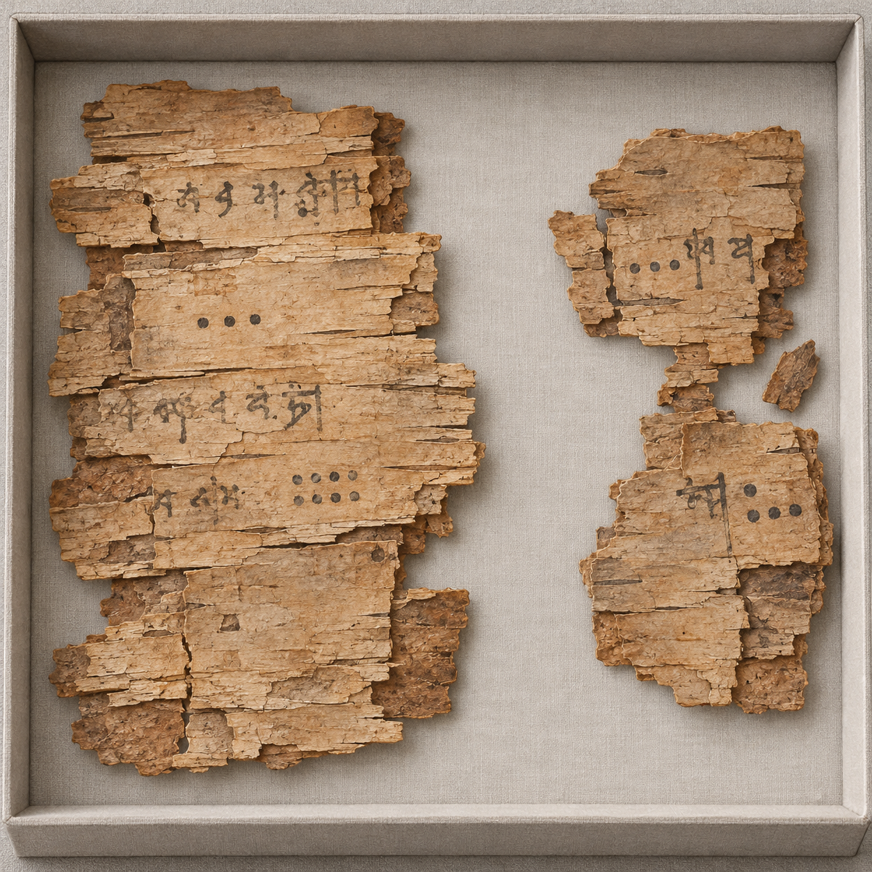
Illustration of imagined birch-bark mathematical manuscript fragments in a conservation tray.
These invented fragments evoke a fragile writing surface; the marks are not a facsimile or a readable mathematical text.

Begin with the mathematics

The manuscript was found in 1881 near Bakhshali in present-day Pakistan and is held at Oxford's Bodleian Libraries. Its surviving birch-bark folios preserve a Sanskrit mathematical work with regional linguistic features. The material is fragmentary, but rules and worked examples give researchers more than isolated numerical symbols.

A worked problem preserves a sequence: state a task, apply a method, obtain a result and sometimes check it. That sequence helps historians investigate what a notation actually does. A dot's appearance is a beginning, while its role inside a calculation supplies further evidence.

Think of a modern exercise in which a blank box stands for an unknown number. Its shape is not enough to tell us its function. The surrounding instruction might ask us to fill the box, add a quantity or compare results. Historical mathematical notation also needs to be read in context.

Three jobs for a small mark

A placeholder distinguishes positions in a numeral. Zero as a number can participate in arithmetic. A symbol can also stand for an unknown quantity. These ideas are related, but they are not identical, and a single visual form can be used within more than one procedure.

In their response to the 2017 dating announcement, historians Kim Plofker and colleagues challenged the description of the manuscript's zeros as merely placeholders. They considered large-number operations and a rule involving substitution for an unknown, arguing that the mathematical procedures complicate such a sharp division.

Their point is valuable even if you do not follow every Sanskrit term. To understand a mathematical symbol, examine the actions performed with it. A claim about the writer's concepts should be supported by the calculations, rather than deduced solely from whether the mark looks like a dot or a circle.

Try a modern comparison. In 105, the zero distinguishes the tens position. In 5 minus 5 equals 0, it is an arithmetic result. In “a number plus 5 equals 12,” an empty space might indicate the unknown 7. These are teaching examples, not transcriptions of Bakhshali problems.

Why the 2017 headline needed revision

Oxford's 2017 announcement drew attention to widely separated radiocarbon results from three pieces of bark, including an early date in the third or fourth century CE. The announcement connected that finding with the history of the zero symbol. Specialists questioned how the samples should be related to the writing and the manuscript as a whole.

A 2024 Oxford report provides later determinations for five folios and a new model. It places the start of the dated bark-formation phase within 799–892 CE and its end within 900–1102 CE, at the stated 95.4 percent probability level. These are modelled boundaries, not two precisely observed days of copying.

The report makes the central distinction explicit: radiocarbon concerns the formation of the bark. Ink must be applied after its writing surface exists, but it can be applied later. The composition of a mathematical rule can be older still, transmitted through copies that have not survived.

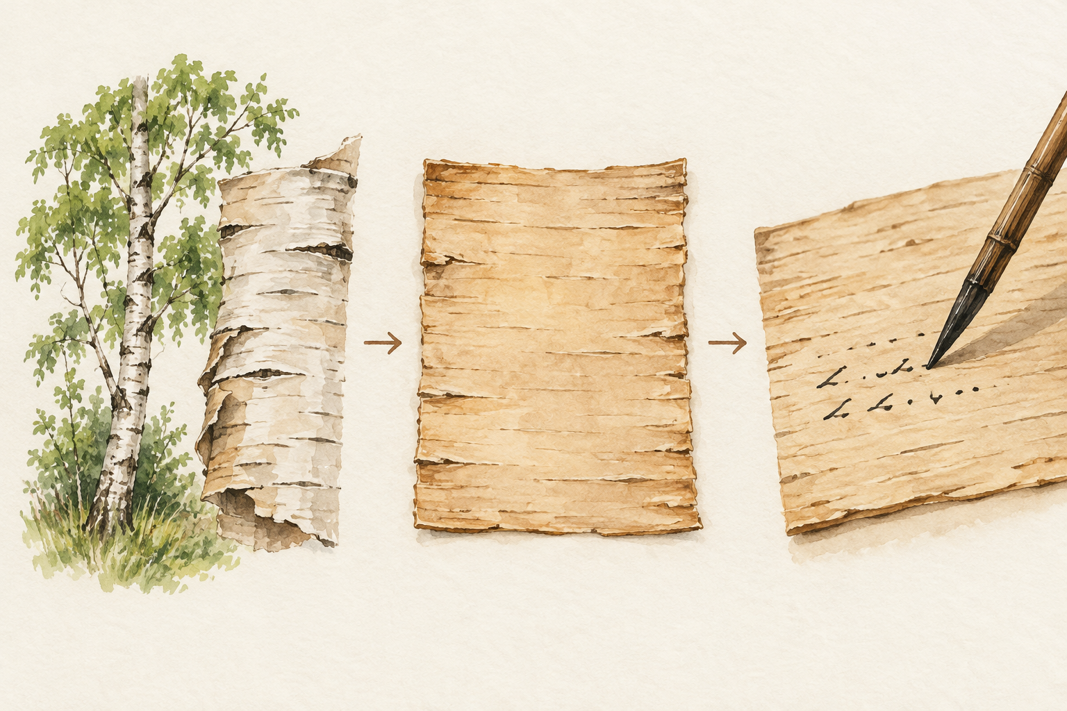
Conceptual sequence from a birch tree to a blank bark sheet and the act of writing.
The surface must exist before it can carry writing. This conceptual sequence does not document the manuscript's exact manufacture.

The layered illustration is a conceptual aid. It does not reproduce a measured folio or assign a time interval between bark formation and writing. That interval has to be investigated with evidence rather than supplied by the attractiveness of a sequence.

A dating exercise with three clocks

Imagine an old notebook copied from an even older textbook. A laboratory tests the paper. A handwriting specialist studies the script. A historian compares the problems with other books. Each investigator can be right while addressing a different date.

Which clock is being read?
EvidencePrimary question
Radiocarbon of barkWhen did this sampled organic material form?
Handwriting and physical structureWhen and how was the surviving copy written?
Comparison of mathematical worksHow were rules and ideas developed and transmitted?

Now test a headline: “The oldest piece of bark gives the invention date of zero.” Which links would have to be demonstrated? You would need a defensible relationship between the sample and the writing, and then between that particular copy and the first development of the idea. The short headline skips both.

That does not make material dating unhelpful. It makes its proper question more precise. Several independent kinds of evidence can strengthen a chronology, especially when a proposed interpretation explains how apparently conflicting results fit together.

Read the report as an argument

Open the 2024 Oxford report record and follow its document link. Look first for the folio identifiers, then for the discussion of modelling. Compare its language with the earlier announcement, keeping the publication dates in view.

The manuscript's value survives that comparison. It remains evidence of people teaching, calculating and checking through a sophisticated mathematical tradition. A later surviving copy can preserve earlier knowledge; an earlier surface cannot by itself establish when every idea was invented. The dot is small, but reading it well requires a generous view of the book around it.

Sources and further reading

Explore more art, stories and discoveries at Incoprea.

Famous Last Meals is now in paperback — stories, history and 25 recipes

Famous Last Meals: Stories, History, and Recipes is now available in paperback on Amazon. The illustrated collection brings together 23 his...