Showing posts with label Computing. Show all posts

Saturday, October 24, 2026

Noise Becomes Useful Randomness Only After You Ask What Could Predict It

Imagine a sensor producing a restless stream of values. The trace looks irregular, so we call it noise. Now suppose a nearby electrical signal nudges every second sample in a predictable direction. The picture can still look busy while the uncertainty available to a computer is smaller than it appears.

A small electronics board sits beneath an irregular luminous amber-and-cyan texture.
A conceptual electronics scene introduces physical noise. It is not a circuit diagram, measured signal, or tested random-bit generator.

Physical randomness is a story about what remains unpredictable under a stated model. Collecting fluctuations, digitizing them, and producing useful bits are different jobs. Their separation explains why a random-bit generator needs more reasoning than a source that merely looks chaotic.

A balanced count can hide a completely predictable rule

Write 010101010101 on a piece of paper. It has equal numbers of zeros and ones, but the next symbol is easy to guess. Now write six zeros followed by six ones. The total is still balanced. A count has preserved one property while overlooking the order.

This makes a good first task: invent three twelve-bit strings with exactly six ones. Give each a different rule. How many samples would a reader need to recognize that rule? You have constructed examples in which an attractive summary statistic says little about predictability.

NIST's statistical-test publication explicitly distinguishes testing from proof that a generator is appropriate for an application. Statistical tests can reveal problems, but they cannot replace a sound account of the generator and its security properties. A few reassuring charts are not a complete explanation.

Processing can concentrate uncertainty without inventing it

NIST SP 800-90B separates a noise source, optional conditioning, and health testing. Conditioning is deterministic processing that can reduce bias or increase entropy per output bit. It cannot repair a source that has stopped providing uncertainty by creating new entropy from nothing.

A small pair rule makes the distinction tangible. Read consecutive, nonoverlapping input pairs. Discard 00 and 11. Turn 01 into 0, and 10 into 1. The output is shorter, and the discarded pairs make the lost quantity visible.

Watch a pair filter keep and discard bits

Deterministic step table exposes bias/dependence assumptions, discarded pairs, and an unfinished trailing bit. No random numbers or security keys are generated.

Open watch a pair filter keep and discard bits in its own window.

Under a specific mathematical assumption—independent input bits with the same fixed probability p of being 1—the probabilities of 01 and 10 are equal: (1−p)p and p(1−p). Among the retained unequal pairs, the two outcomes are equally likely. That argument relies on the assumption. It does not prove arbitrary physical samples satisfy it.

Use the preset repeating input 010101010101. The pair rule emits only zeros. The input was balanced, yet dependence defeated the informal promise that a filter would make everything fair. Next use 00111001. Its pairs are 00, 11, 10, and 01; only the last two survive, giving 10.

The same assumption also predicts an efficiency cost. Unequal pairs occur with probability 2p(1−p). At p = 0.9, only 18 percent of pairs survive on average, producing one output bit per retained pair. That is an expected output length of 9 percent of the input bit count, not a guaranteed result for a short sequence.

Keep the raw evidence available

The filter demonstration is entirely deterministic: it processes the text you enter and generates no physical randomness. That limitation is the point. A clean-looking output cannot tell you everything about the source that produced the input. Reviewing raw behavior and its physical origin can expose failures that later processing obscures.

Imagine a sensor that is stuck at one value. A monitoring system should notice the failure rather than keep issuing a reassuring status because another part of the device is still running. In a real design, the monitoring rules must suit the source and the failures it can experience.

NIST and BSI's discussion of tailored health tests addresses that source-specific work. The presentation distinguishes observing a source's operation from merely assessing a finished bitstream. Different physical mechanisms can have different ways of going wrong.

Make a claim small enough to defend

Take the sentence “These bits are random.” Replace it with four questions: What physical process supplies uncertainty? How are samples taken? What assumptions support the estimate? What happens when the source fails? Each question asks for a different kind of evidence.

A useful pair-filter challenge

Predict the output before pressing Process. Then count input bits, discarded pairs, retained pairs, and any trailing unpaired bit. Try an odd-length input. The unfinished bit must remain unused rather than silently receiving a fabricated partner. Try all zeros, then the alternating preset. Both produce warnings for different visible reasons.

The most interesting part of a useful random source is often the discipline around it. Engineers do not merely collect disorder. They decide which uncertainty can be credited, what processing preserves it, and how an apparently lively machine will reveal that it has become predictable. The question behind the noise is always: predictable to whom, with which information?

Sources and further exploration: NIST SP 800-22: statistical testing and its limits; NIST SP 800-90B: entropy-source design; NIST and BSI: tailored health tests.

Explore all 50 new articles · Browse the complete illustrated collection

Explore more art, ideas, and independent projects at Incoprea.

Friday, October 23, 2026

The Music Disc Whose Pits Are Not Simply Ones and Zeros

Hold a music CD by its edge and its surface seems almost featureless. Tilt it and a rainbow arrives. Somewhere in that reflective object is an ordered account of sound, but the convenient story that “a pit means one and a flat place means zero” skips the part that makes the system readable.

Illustrated silver compact disc above an enlarged optical pickup on a dark blue surface.
The pickup and light path are enlarged and shown in visible color for clarity; an actual CD reader uses near-infrared light.

A pressed compact disc is not a tiny vinyl record. Its microscopic relief does not imitate the shape of the original sound wave. A pickup reads changing reflected light, and a chain of decoding operations reconstructs digital information. The physical pattern is the beginning of that chain, not its final meaning.

A shape, an optical signal, and a code

The NIST optical-disc guide describes replicated discs whose pits and lands are molded into a polycarbonate substrate and covered by a reflective layer. The reader focuses laser light through the disc and detects the returning signal. Tracking follows a spiral rather than a stack of independent circular grooves.

Now separate three descriptions. The surface has physical relief. The pickup produces a varying electrical signal from reflected light. The electronics interpret that signal according to coding and timing rules. A feature at the first level does not automatically equal a user-data bit at the third.

Look for the change

In the channel recording described by ECMA-130, section 19.4, a channel ONE corresponds to a transition between pit and land, in either direction. A channel ZERO corresponds to no transition. A long pit can therefore contain several channel intervals without becoming a row of user-data ones.

Those are still channel bits. The standard's eight-to-fourteen modulation maps eight-bit values into fourteen-channel-bit patterns, with additional merging bits between them. The channel patterns restrict the spacing of transitions. Framing and error-correction information belong to the larger decoding process. Audio-CD details are specified separately, a distinction the CD-ROM standard itself makes.

Read a transition-coded toy track

Toggle bits and compare state versus transition; explicitly not a full EFM encoder.

Open read a transition-coded toy track in its own window.

Our small reader strips the problem down to one rule: a change at a clock boundary is a one; staying in the same state is a zero. Toggle a channel bit and watch what happens to all the physical states that follow. This demonstration is not a valid EFM encoder. It intentionally omits the run-length, synchronization, and error-correction requirements of a real disc.

Conceptual enlarged spiral track with alternating elongated pits and flat lands.
A state is not the same thing as a transition. This enlarged track is an interpretive view, not a measured micrograph.

Try decoding this imaginary track

Start in a land state. At successive clock intervals the channel pattern is 10010001. The first one changes state to pit. The next two zeros keep the state unchanged. The next one changes it back to land. Work through the remaining intervals before revealing the result.

Reveal the state sequence

The successive states are pit, pit, pit, land, land, land, land, pit. There are three transitions. Saying “every pit is a one” would lose both their timing and the distinction between a state and a change of state. This short pattern illustrates transition decoding only; it is not a complete legal CD frame.

A homemade recordable disc is a different object

A CD-R uses a recording layer whose optical properties are changed during writing; a rewritable disc uses another recording technology again. These media are made to produce readable optical changes, but that does not make their internal construction identical to a molded, factory-pressed disc. The Canadian Conservation Institute's guide separates read-only, recordable, and erasable media.

This distinction helps when you look at an old collection. The format name, visible label, recording history, and ability to read the contents are different pieces of evidence. A shiny surface is not a complete condition report. Nor does success in one drive establish indefinite future readability.

The remarkable achievement is coordination across scales. A microscopic relief pattern becomes a timed optical signal, a constrained channel code becomes recovered data, and data becomes something a listener recognizes as music. The disc can look silent and simple because the reader knows a great deal about how to interpret it.

Follow the evidence: Ecma International: ECMA-130; NIST: care and handling of CDs and DVDs; Canadian Conservation Institute: recording media.

Explore all 80 new articles · Browse the complete illustrated collection

Explore more art, ideas, experiments, and independent projects at Incoprea.

Thursday, October 22, 2026

The QR Code Can Lose Pieces and Still Speak

A coffee stain can cover part of a QR code and the phone may still read it. That small success hides two different problems. First the reader has to find and geometrically interpret a square in a messy view. Then it has to recover a message whose visible marks may contain mistakes. A code that solves only the second problem might still be unreadable.

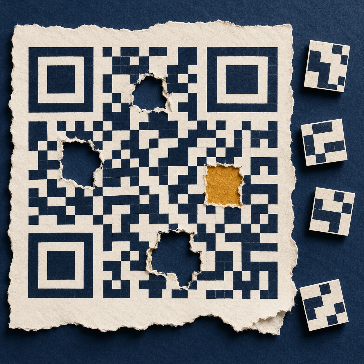
A deliberately nonfunctional code-like matrix with torn patches and conceptual reconstruction tiles.
Conceptual artwork, not a scannable QR code or a demonstration of a particular correction threshold.

The extra information is not merely the same web address printed repeatedly. The message is encoded with mathematical redundancy: relationships among codewords that allow a decoder to detect and correct certain errors. A codeword is a group of bits, not one black square. The distinction matters whenever someone claims a logo can safely cover a particular fraction of an image.

What the familiar percentage actually describes

DENSO WAVE's error-correction explanation identifies Reed–Solomon coding and four levels of protection. The commonly quoted approximate restoration levels—L 7%, M 15%, Q 25% and H 30%—refer to total codewords, not a guarantee that any matching percentage of the printed area can be erased.

Where damage lands matters. So do the geometry and the pattern that a reader must locate before decoding. A rectangle over a critical locating feature is not equivalent to the same number of damaged data modules spread elsewhere. Error correction is a designed capacity within a reading system; it does not make that system indifferent to its input.

Here is a separate, much simpler analogy. Write three numbers and a check total: 4, 7, 2; total 13. If one number is known to be missing, subtracting the other two from 13 recovers it. But if a number is merely wrong and you do not know which one, that single check does not identify the problem. Real error-correcting codes use more powerful relationships. The example shows why detecting a mismatch, locating an error and rebuilding a value are different achievements.

One more relationship can reveal where a change occurred

The earlier three-number example can recover a known missing value. Extend it with a second relationship and it can do something more interesting under a tightly stated assumption: identify one changed slot.

Phone held above a tilted abstract black-and-white matrix card on a library table.
The matrix is deliberately nonfunctional. It illustrates the reading task and contains no test message.

Keep the original values 4, 7 and 2. Their ordinary total is 13. Also store a weighted total: once the first value, twice the second, three times the third. That gives 4 + 14 + 6 = 24. The position of each number now affects one check differently.

Suppose the received values are 4, 9 and 2. The ordinary total has increased by 2; the weighted total has increased by 4. If exactly one data value changed and the checks remained intact, the ratio of those changes identifies the position: 4 ÷ 2 = 2. The second slot increased by 2, so its corrected value is 7.

This is an original ordinary-number puzzle, not the mathematics used inside a QR code. DENSO WAVE's explanation identifies byte-level Reed–Solomon coding, and William Geisel's NASA tutorial develops the field arithmetic and error-location machinery needed for that real system. The simple puzzle lets you encounter the job of an additional relationship without pretending to implement it.

Find a changed number with two checks

Print-friendly arithmetic puzzle with a single-error solution and a multiple-error counterexample.

Open this activity in its own window.

The assumption is part of the solution

The worksheet includes a second received message in which two values changed. Applying the single-error shortcut then produces a confident correction that satisfies both checks but recovers the wrong original message. Try it before opening the explanation.

That failure is useful. It shows why a correction method must be judged within its designed error capacity. A decoder is not making a philosophical promise that every plausible message is the intended one. It is using a particular code, a set of relationships and limits on the damage it can resolve.

Bring this distinction back to the stained square. Locating the symbol, identifying errors and reconstructing data are cooperating tasks with different assumptions. A successful scan feels immediate because those stages are hidden. Slowing down one tiny arithmetic version makes the hidden work much easier to appreciate.

The square has to announce itself first

In the developer's history, Masahiro Hara's team focused on finding a symbol quickly, rather than maximizing capacity alone. The prominent position patterns were designed to be distinguishable from surrounding printed matter. Their black-and-white run ratio helps the reader recognize a candidate code at different orientations.

That design choice gives a useful lesson for people making posters: the parts that seem like decorative framing are doing work. Treating the three conspicuous corner patterns as spare space misunderstands their job. A human may still recognize “something QR-like” after an alteration, while the decoder has lost the geometry it needs.

The empty space outside the code also counts. The official layout guide specifies a clear quiet zone four modules wide on every side for a standard QR code. The white border is part of the reading conditions, even though it contains none of the message.

More protection has a cost

The official version guide explains that a symbol's capacity depends on its version, character mode and correction level. Version 1 has 21 modules per side; subsequent versions add four per side, up to Version 40 at 177. Increased protection uses capacity that could otherwise hold message data. For a fixed message, the needed version can therefore increase.

Imagine two posters with the same physical square size. If one symbol needs more modules, each module becomes smaller. The extra mathematical protection may be useful, but printing and focusing now have a more demanding pattern to resolve. “Choose the highest level” cannot replace checking the finished print under intended conditions.

You can do a layout calculation without a phone. Suppose a chosen symbol has 29 modules per side and you allot 0.5 millimeters to each module. Its patterned square is 14.5 millimeters wide. Including four quiet-zone modules on each edge adds eight modules, so the total allocation is 37 × 0.5 = 18.5 millimeters. That is a geometry example, not a recommended minimum size for every application.

A successful read is only the first success

A QR code may contain a web address. Recovering the characters does not demonstrate that the destination still exists, that a redirect is dependable, or that the page is useful on a phone. The printed symbol and the service behind it have different lifetimes. A good publication check follows the whole experience from paper to readable content.

This is the deeper reason the battered square is interesting. It joins recognition, geometry, error correction, manufacturing and a reader's task in one small object. Its resilience comes from anticipating imperfect conditions at several levels. The coffee stain is simply where that preparation becomes visible.

Sources and a closer look: DENSO WAVE: error correction; DENSO WAVE: development history; DENSO WAVE: quiet zone and print area; DENSO WAVE: versions and capacity.

Explore art, experiments and other unexpected connections at Incoprea.

The Camera That Records Different Moments in One Photograph

A conceptual street scene is assembled from horizontal strips to evoke line-by-line timing.
Temporal collage. It illustrates an idea, not a camera test or an actual captured rolling-shutter example.

A straight post leans in a photograph taken from a moving train. A propeller seems to bend into disconnected blades. The easy explanation is “the camera was too slow,” but that phrase hides two different times. A row of pixels may have a very short exposure while the whole image still spans a longer sequence of moments.

Rolling shutter is the process that makes those moments coexist in one rectangular frame. Different rows begin collecting light at different times. If the subject or camera moves between them, the finished image assembles a shape that no single instant contained. The sensor has recorded a timetable as well as a view.

Short exposure does not mean simultaneous exposure

Basler's technical documentation describes the row-to-row temporal offset. In a conventional rolling sequence, the first row starts, then the next begins after a delay, and the process continues across the selected image region. Each row can have the same exposure duration while occupying a different interval on the clock.

Picture a person surveying a building through a narrow horizontal slot. They draw the roof first, the middle later and the foundations last. If the building moves sideways during the survey, the copied roof and foundations belong to different positions. Their drawing may be sharply rendered in every strip and still fail to represent one undistorted building.

By contrast, a global exposure aligns the integration interval across the image. That does not abolish motion blur: a moving object can still travel during a long exposure. It changes whether all image locations share the same interval. Blur within an interval and geometric displacement between intervals are different effects.

Build a frame out of times

Use a deliberately simple numerical example. Suppose the first row begins at 0 milliseconds and the last at 20 milliseconds. Every row exposes for 1 millisecond. An object moving sideways at 1,000 image pixels per second shifts 20 pixels between the first and last starting times, although it moves only one pixel during each row's individual exposure.

Those invented values are not a measurement of a phone. They show why changing the exposure from 1 millisecond to 0.5 millisecond does not automatically remove a 20-millisecond scan interval. The strips can become sharper while the assembled object's lean remains. To change the lean, one must also consider row timing and motion.

QuestionTime quantity to inspect
Why is a moving edge smeared?How far it moves during each pixel's integration interval
Why do straight edges lean?How far the scene shifts between row exposures
Why do successive frames differ?How camera motion and acquisition timing vary from frame to frame
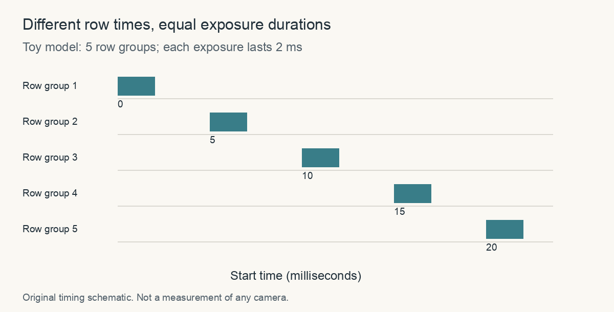
Five row groups begin at 0, 5, 10, 15 and 20 milliseconds; every exposure lasts 2 milliseconds.
Original timing schematic: the equal-width bars represent equal exposure durations starting at different times. These invented values do not describe a particular camera.

The geometry is a research problem too

In Geometric Models of Rolling-Shutter Cameras, Marci Meingast, Christopher Geyer and Shankar Sastry developed projection equations that account for different camera motions. Their point was larger than a funny propeller image: treating a rolling frame as one instantaneous central projection can bias estimates of scene geometry and camera motion.

A photograph used for reconstruction is therefore a measurement whose acquisition model matters. The same visual artifact that makes a vacation image amusing can become a systematic error when software uses many such images to infer the shape of a room. The answer is not to call all distorted images useless, but to understand the timing assumptions of the method.

A shared pulse of light needs a shared window

There is a surprising way to separate the electronic exposure schedule from the light that actually contributes to the image. Different rows may be open over different intervals, yet share a shorter interval during which all are open together. A carefully controlled pulse within that overlap can illuminate them at the same time.

Digital camera on a tripod facing a caged tabletop fan in a softly lit studio.
Conceptual camera-and-subject scene. It is not a captured rolling-shutter test, timing measurement, or setup instruction.

Basler's flash-window documentation defines this common interval for supported cameras. In a conventional rolling sequence, it begins when the final row starts exposure and ends when the first row finishes. It exists only if those events occur in that order.

Find the overlap on paper

Consider five fictional row groups starting at 0, 5, 10, 15 and 20 milliseconds. If each exposes for 25 milliseconds, their intervals are 0–25, 5–30, 10–35, 15–40 and 20–45. Which time range lies inside all five?

Check the common interval

It runs from 20 to 25 milliseconds, a five-millisecond overlap. A short pulse entirely inside it reaches every row during its exposure. If each row instead exposes for only three milliseconds, there is no common interval.

These invented times are a reading model, not settings for a camera or an instruction to flash a lamp at a spinning object. Real use depends on the supported sensor, synchronization and control of other illumination. Continuous ambient light can still contribute during the rest of each row's exposure.

A second Basler note on exposure-end events shows why even a timestamp's name needs checking. In the described older ace behavior, the event refers to the first row's readout rather than the completion of the whole image region. The note distinguishes that behavior from ace 2. One label cannot be interpreted identically across every model.

When reading a timing diagram, mark three things in different columns: electronic integration, illumination, and the reported event. Their intervals may overlap without being identical. The camera-and-fan illustration supplies context for the question, rather than an experimental result.

A photograph's history is therefore more than a shutter-speed number. The acquisition schedule decides when the material can respond; the lighting decides when useful photons arrive. Understanding both reveals why a clever measurement can change the effective moment without turning the sensor into a different kind of device.

Why use a rolling shutter at all?

Basler's engineering introduction explains why rolling designs can be useful for stationary or slowly moving inspection tasks. Sensor architecture affects sensitivity, noise, cost and readout. A design chosen for one application can be a good tradeoff even if it produces unwanted geometry in another.

Sony's account of its industrial sensors similarly discusses pixel design and column-parallel conversion as routes to low noise and sensitivity. Those are descriptions of particular technology families, not a universal ranking in which every rolling sensor outperforms every global sensor. The acquisition task defines which properties matter.

A camera does not merely decide which photons belong to a photograph. It decides when each part of that photograph happens. The leaning post is a visible trace of that hidden schedule. Once you know to look for it, “a picture of a moment” becomes a more interesting and more conditional phrase.

Sources and a closer look: Basler: electronic shutter timing; Meingast, Geyer and Sastry: rolling-shutter projection models; Basler: rolling-shutter camera design; Sony: industrial rolling-shutter technology.

Explore art, experiments and other unexpected connections at Incoprea.

Wednesday, October 14, 2026

The Jacquard Card Chain: A Textile Pattern Stored in Holes

A complicated textile can begin as a long chain of small decisions: lift this group of threads, leave that group down, pass another thread through, then change the selection. In a Jacquard mechanism, a sequence of punched cards helps make those decisions repeatable. The pattern is stored outside the weaver's memory and presented to the mechanism one step at a time.

The holes are immediately intriguing. Follow them into the rest of the system, though, and a richer story appears: the work of designing a pattern, preparing cards, keeping a sequence in order, and turning that sequence into cloth. It is a story about labour and materials as well as information.

A generalized wooden loom has a hanging punched-card chain and patterned burgundy-and-cream cloth.
An invented historical weaving scene combines a Jacquard-style card chain and cloth. It is not an exact museum machine or a diagram encoding the depicted textile.

What the card controls

The warp is the set of threads held along the loom. The weft passes across them. To weave a patterned structure, selected warp threads or groups have to be raised in a particular sequence. The Jacquard attachment provides a way to control that selection using information carried on cards.

In a simplified account, a hole permits one action while the absence of a hole produces the alternative. The actual relationship between a card position, hooks and threads depends on the loom's arrangement. “One hole equals one thread” is therefore a poor universal rule. The important point is that a physical difference is read by a mechanism.

Illustrative close-up of a linked punched-card chain, showing perforations, lacing and the scale of a nearby hand.
An illustrative close-up of a card chain. Its holes do not encode a verified historical textile pattern.

Follow the joins in this close view, rather than counting the holes. Which details let separate cards travel as a sequence? Imagine turning one card around or putting it in a different position. The perforations would remain, but their relationship to the machine and the neighbouring cards would change.

A card does not contain a picture in the way a photograph contains one. Its significance depends on its position in the chain and on the apparatus that interprets it. Without those relationships, a perforated rectangle is only a perforated rectangle. Stored information needs an agreed way to become an action.

Follow a real chain through a museum object

National Museums Scotland describes a handloom used for silk weaving in Stonehouse, Lanarkshire. Its Jacquard attachment worked with cards laced together, potentially in their thousands, to produce complex designs. The museum names the brothers Robert and James Hamilton as its users and records a maker's stamp associated with Joseph Hood of Newmilns.

Those details return people and places to a machine often presented only as a milestone on the road to computing. A loom had to suit a workshop, materials, a market and workers who knew how to use it. The surviving object also carries a regional industrial history.

Look at the museum's gallery photographs in sequence. Start with the entire loom, then the hanging cards, then the cloth. Where does the stored pattern enter? Where is motion transmitted? Where does the product emerge? Moving among these views is more informative than trying to understand everything from a single dramatic photograph.

The holes had to be made

The Science Museum Group holds a card-making hole punch made in Coventry in 1870 by James Heywood, catalogued as part of a model. It directs attention to an easily missed stage: instructions have to be prepared before the loom can use them. Mechanisation redistributes work; it does not make the work of design vanish.

A pattern must become a sequence the particular machinery can read. Card positions need to correspond to intended selections, and the cards need to stay in the right order. Repeating a pattern reliably becomes possible because a great deal has been specified in advance.

This changes the nature of an error. A faulty selection may recur whenever the same card returns. A misplaced card can disrupt the sequence. A mechanical fault may produce a different kind of problem. To understand a flaw in the cloth, a worker needs to consider both the instructions and the apparatus that carries them out.

A small sequencing puzzle

Imagine a demonstration with only four controlled thread groups, named A, B, C and D. The following table gives selections in words. It is an invented teaching example, not a card design for a historical loom.

Four successive selections
StepGroups selected
1A and B
2B and C
3C and D
4D and A

First imagine that step two accidentally selects D as well as B and C. Then imagine that the cards for steps two and three have been swapped. Both faults alter the result, but they alter different things. One changes the content of an instruction; the other changes its place in the sequence.

What should you inspect first?

For an unwanted selection that appears at the same point in each repeat, inspect the relevant card and the mechanism it controls. For two otherwise plausible selections arriving in the wrong order, inspect the chain's arrangement. This is a reasoning exercise, not a diagnosis for operating machinery: real looms can have several interacting faults.

The point is to notice that order is itself information. A bag containing all the correct cards cannot do the work of a correctly arranged chain. That principle carries far beyond weaving, but it is already tangible here in the links between neighbouring cards.

Watch the textile before following the computer connection

The Science and Industry Museum's article “Weaving numbers” includes a film about the loom and early computing. On a first viewing, follow the cards and the repeated mechanical movement. On a second, focus on the threads and the emerging fabric. The two views connect an abstract sequence to a material result.

Charles Babbage proposed punched-card input for his Analytical Engine. The Science Museum's drawings show cards within a broader planned calculating system. That connection is substantial, but the textile mechanism was not itself a general-purpose computer, and a drawing of the Analytical Engine is evidence of a design rather than a completed Victorian machine.

The most useful inheritance is a way of thinking: instructions can be stored in a durable physical form, read in sequence, and used to govern repeated operations. The cards make that idea visible. The cloth reminds us why it was developed and why the people who prepared, read and worked with those instructions belong in the story.

Sources and further reading

Explore more art, stories and discoveries at Incoprea.

Magnetic Core Memory: The Computer That Restored a Bit After Reading It

An artistic macro view of dark ferrite rings and fine wires within a memory-like metal frame.
An artistic detail of ferrite rings and woven wiring. It is not an identified historic artifact or an exact core-plane wiring diagram.

Before memory became a collection of microscopic devices on a silicon chip, a computer could remember with tiny magnetic rings. Viewed close up, a core-memory plane resembles an intricate woven surface: wires threaded through ferrite rings, each carrying a small piece of information.

The construction makes a digital idea unusually tangible. A bit has a place in a physical grid, and changing a magnetic state changes the information stored there.

One ring can represent one bit

A core can be magnetized in two opposite directions, assigned the meanings zero and one. A plane contains many such cores, with wires arranged to select and operate on them. The wire network is essential to the memory, rather than merely a way to fasten its parts together.

The Computer History Museum places core memory in MIT's Whirlwind computer in 1953. It credits Jay Forrester with perfecting the technology while acknowledging that several inventors contributed to its development.

The underlying idea separates a value from its ordinary appearance. A ring need not visibly change color or position when a bit changes. Electronics create and detect the magnetic condition that encodes the value.

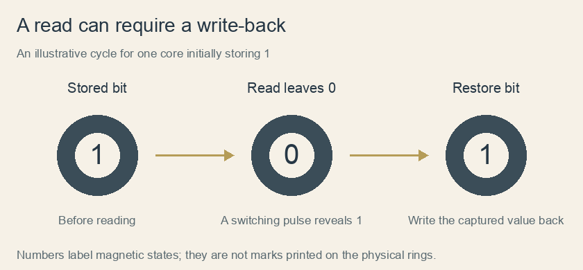
Three stages show a core holding one, a read leaving zero while detecting the former one, and a write-back restoring one.
Original logical schematic of a destructive-read cycle for a core initially storing 1. The displayed digits label magnetic states, not physical markings. The diagram omits circuitry and timing details.

How does a grid choose just one ring?

Imagine a square of paper with four rows and four columns. Mark one crossing in the second row and third column. Running a wire through each row and another through each column gives the circuit a way to address that crossing without dedicating an entirely separate pair of wires to every ring. The challenge is to disturb the chosen ring while leaving its neighbors alone.

Coincident-current selection exploits a switching threshold. A pulse along the row is insufficient by itself to reverse a core; a pulse along the column is also insufficient. At their selected intersection, the combined magnetic effect can be sufficient. Cores elsewhere along either selected line receive only the smaller effect. Real hardware needs careful tolerances and pulse timing, but the paper grid reveals why selection can scale beyond a handful of bits.

Try tracing both selected lines with a pencil. How many rings lie on either line, and how many sit at their intersection? The distinction between receiving a partial disturbance and actually switching is the ingenious part. Physical access to a wire does not automatically mean access to every stored value on that wire.

Reading changes what is stored

Ken Shirriff's direct examination of an IBM 1401 core module explains a particularly surprising feature. Selected currents in crossing address wires operate on the chosen core. During a read, the circuitry drives it toward the zero state.

If the core previously held one, switching its magnetization produces a signal in a sense wire. If it already held zero, that switching signal is absent. The electronics can distinguish the former value, but the read has left the core at zero.

The system therefore writes the desired value back. “Destructive read” describes this controlled change of state, rather than physical damage to the ferrite ring. Reading and restoring are cooperating parts of the memory operation.

The process turns measurement into an active event. The circuit learns a value through a change, then uses the captured result to restore the information.

A read cycle, reconstructed one bit at a time

Start with a written sequence, 1–0–1–1. On a second line, record the sense result as you pretend to drive each selected ring toward zero. A ring initially holding one supplies the switching indication; a ring initially holding zero does not. After four reads, your imaginary cores all hold zero, while your second line preserves the information that the sensing circuit captured.

Now restore the original sequence from that second line. This small bookkeeping exercise separates three things that are easily merged in a verbal explanation: the original magnetic state, the signal generated during a transition, and the state remaining afterward. The signal is evidence of what happened, not a tiny numeral taken out of the ring.

Suppose the restore step were skipped only at the third position. The next read of that position would report zero, even though no ring had cracked and no wire had disappeared. This is why the title's word “restored” refers to information. Destructive reading is an intended electrical operation with a necessary companion operation, rather than wear caused by looking too often.

A useful final distinction concerns power. A core's magnetic orientation can persist without continual electrical refreshing. That does not make an interrupted read cycle harmless: the circuitry still has to complete its work correctly. Remembering a state without power and preserving that state through every operation are different engineering requirements. Semiconductor memories likewise use different mechanisms; “computer memory” names a job rather than one universal physical process.

Manufacturing mattered as much as the clever bit

IBM's history of dynamic random-access memory describes magnetic-core storage in the mid-1960s as arrays of hundreds of thousands of ferrite elements laced with thin wires. By then, assembly had become highly automated.

That detail corrects the tempting image of an entire era depending exclusively on people threading every ring by hand. The technology developed along with methods for producing it, while its density, cost and performance still faced practical limits.

Semiconductor approaches offered a route to placing memory elements on chips. Robert Dennard's work on dynamic memory used a different storage arrangement, with charge and an integrated device taking the role previously served by an individually wired magnetic core.

The older grid remains fascinating because it exposes the physical work behind remembering. Its rings show how a computer's abstract zeros and ones can arise from material states, carefully selected currents and a sequence that even includes repairing the information after it has been read.

Sources and further reading: Computer History Museum: Memory and storage timeline · Ken Shirriff: Direct examination of IBM 1401 core memory · IBM: Magnetic-core manufacturing and the development of DRAM · Computer History Museum: Whirlwind and magnetic-core storage

Famous Last Meals is now in paperback — stories, history and 25 recipes

Famous Last Meals: Stories, History, and Recipes is now available in paperback on Amazon. The illustrated collection brings together 23 his...