To take the ocean’s temperature, you can lower an instrument into it. Or you can send a sound across a large region and measure how long the journey takes. The second approach turns a route through the sea into a thermometer with an unusual shape.
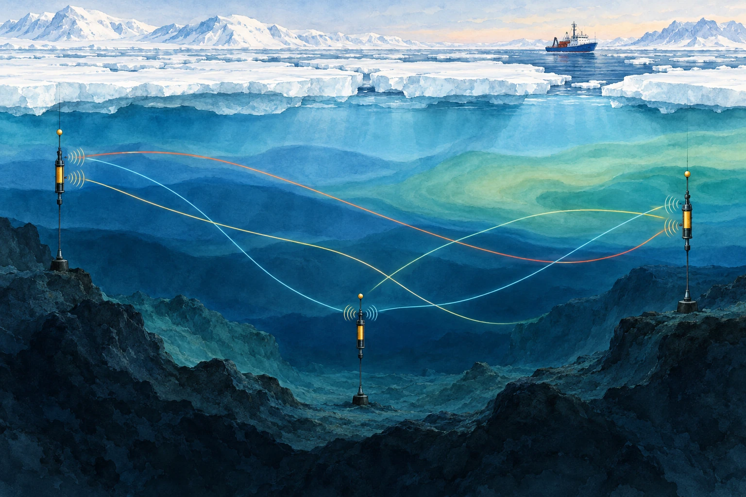
Ocean acoustic tomography uses travel times between known sources and receivers to infer properties of the intervening water. Its strength is also its interpretive challenge: the measurement integrates conditions along a path, rather than reporting the temperature at one point.
Time is the measurement
Sound speed depends on temperature, pressure, and salinity. In many ocean settings, temperature changes make an important contribution to travel-time variations. If the water along a known route becomes acoustically faster, a signal tends to arrive sooner, though currents and changing paths must also be considered.
WHOI’s ocean-acoustics overview describes tomography as an inverse problem: use measured travel times and known instrument locations to estimate the ocean properties responsible for them. A received pulse is not an underwater thermal photograph.
The appeal is coverage. A long acoustic path can sample a large region quickly and repeatedly. A point thermometer may be exquisitely accurate but describe only its immediate surroundings. The two approaches answer complementary questions.
The same arrival can hide different oceans
Suppose a route crosses two equal-length regions. One could warm while the other cools, leaving the overall travel-time change small. A different route that crosses only the first region could reveal the imbalance. Several crossing paths provide more information than one long connection.
This is the logic of tomography: overlapping integrals constrain a spatial pattern. The reconstruction still depends on the observing geometry, prior information, and the range of structures the available data can resolve.
Munk and Worcester’s early account of ocean acoustic tomography explains the proposal to use travel times among moorings for mapping. The method’s elegance lies in turning the ocean’s acoustic propagation from a complication into a quantitative observation.
A timing calculation
For a deliberately simple straight path of 1,000 kilometers and a uniform sound speed of 1,500 meters per second, the travel time is about 666.7 seconds. Increase that hypothetical speed to 1,501 meters per second and the time becomes about 666.2 seconds—a change of roughly 0.44 seconds.
Those round numbers are not an actual experiment or a temperature calibration. They show why precise clocks can detect a small fractional change accumulated over a long route. Converting the result to temperature requires the appropriate sound-speed relationship and an account of pressure, salinity, currents, and path geometry.
It also explains why source and receiver motion matters. A mooring that shifts changes the distance. If that shift is ignored, the analyst may assign its timing effect to the water instead. Surveying and position estimation belong inside the measurement chain.
Send sound both ways
A current can help sound travel in one direction and oppose it in the other. Reciprocal measurements—sending between two endpoints in both directions—can help distinguish a shared sound-speed contribution from an along-path flow contribution.
In an idealized uniform example, add a small current speed to the sound speed for the downstream trip and subtract it for the upstream trip. Their mean and difference then contain different information. Real analyses account for ray geometry and variable currents; the simple arithmetic is a conceptual doorway, not the full inversion.
Accurate reciprocal comparison also requires attention to timing. If the ocean changes substantially between transmissions, the paths are not sampling identical conditions. A carefully designed schedule is part of making the separation meaningful.
Two directions can separate two unknowns
In the uniform example, the downstream travel time is L/(c+u) and the upstream time is L/(c−u). Here L is path length, c is sound speed relative to water, and u is current along the route. The signs describe one simplified geometry, with a current that remains steady while both measurements are made.
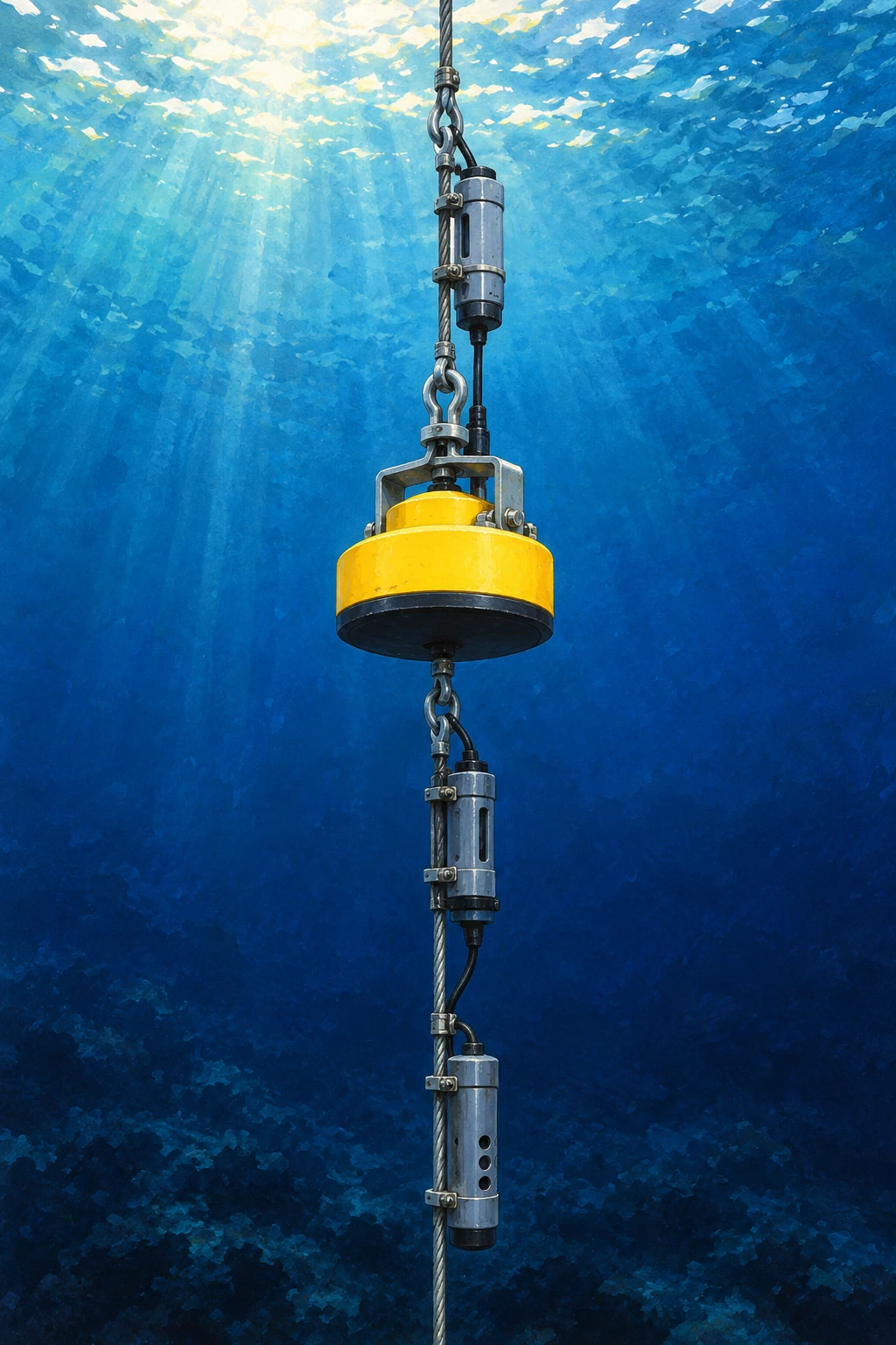
Munk, Worcester, and Wunsch’s chapter on currents develops the reciprocal-travel-time idea in its fuller oceanographic setting. Worcester’s review of experimental work documents the effort to test temperature and current measurements against actual observing conditions. The elementary equations below are an entry point, not a substitute for those experiments.
Let the current reverse
For an invented 300-kilometer route with c=1,500 meters per second and u=1 meter per second, the two travel times are about 199.867 and 200.133 seconds. Their difference is roughly 0.267 seconds. Reverse u and the earlier arrival switches direction, while the common sound-speed term remains nearly the same.
Let the current reverse
Exact uniform-path reciprocal times and reconstructed c,u from hypothetical inputs.
The model also calculates c and u from the two reciprocal times using the exact uniform-path relationships. Change sound speed while leaving the current fixed. Both times shift together. Change current while leaving sound speed fixed. The directional contrast becomes more prominent. Those different signatures explain why two-way observations add information.
A careful limitation is visible even here: the arithmetic assumes the same route length in both directions. In a real ocean, refracted paths, moving moorings, changing water, and the transmission schedule can complicate that symmetry. Travel time is precise only if its physical interpretation is comparably careful.
For a final puzzle, imagine that the upstream trip was recorded after the current strengthened. Can you still interpret the pair as one simultaneous uniform state? You can compute a number, but the assumptions no longer match the situation. A mathematically exact inversion of an unsuitable model can give a physically misleading answer.
That is why the return journey is so useful and so demanding. It provides a second observation designed to respond differently to two properties of the same water. The ocean becomes measurable through a comparison whose geometry, timing, and limits are kept in view.
Why the Arctic is an especially interesting place to listen
Sea ice complicates access for ships and some satellite observations of the underlying ocean. Sound can cross beneath it. A 2026 Scripps report describes research using acoustic travel times to track Arctic ocean temperatures under the ice, providing a way to study variability in a difficult environment.
Read that capability as a complement to other measurements. Instruments that profile temperature and salinity help constrain the inversion; acoustic observations add broad path coverage and repeated sampling. An acoustic average is useful precisely because it is different from a single profile.
A reported “temperature change” should specify the depth range, region, weighting, and uncertainty. Without those details, two observing systems may appear to disagree when they actually sampled different parts of the ocean.
Paths are bent, and sometimes supplied by earthquakes
NOAA’s sound-propagation guide explains why vertical sound-speed gradients bend acoustic routes. A transmission can produce multiple arrivals associated with different paths. Correctly matching arrivals over time is therefore an essential analysis step.
Researchers have also explored using naturally generated ocean sound associated with earthquakes. Work on vertical-slice tomography with seismic waves investigates what changing travel times from repeat sources can reveal. Natural sources offer opportunities but bring their own source-location and repeatability questions.
The family resemblance is the inverse problem: establish what traveled, where, and when before assigning a change to the medium. A natural signal is not automatically simpler because no research transmitter was deployed.
A map-reading exercise
Draw three source-receiver paths across a rectangle. Mark a small warm patch crossed by only one route, then a broad patch crossed by all three. Which pattern would be easier to distinguish from the available travel times? Add two more paths and see how the answer changes.
Finally shade the regions with no crossing paths. A smooth reconstruction might still color them, but the observations constrain them less directly. That gap between a complete-looking map and uneven information is one of the most useful things to notice in any inverse image.
The ocean’s temperature is not written on the sound like a label. It is inferred from a journey, using physics, geometry, and careful comparison. The listening becomes powerful because the uncertainties are part of the account.
Sources and a next step
- WHOI: ocean acoustics and inverse problems
- Munk and Worcester: ocean acoustic tomography
- Scripps 2026: acoustic Arctic temperature measurements
- NOAA: sound propagation in the ocean
- Callies et al.: tomography with seismic waves
Continue exploring art, ideas, and unexpected connections at Incoprea.