A star can look steady while its brightness carries many small oscillations at once. The changes overlap. Watching one rise or dip is much less informative than recovering the pattern of frequencies that produced the changing light.
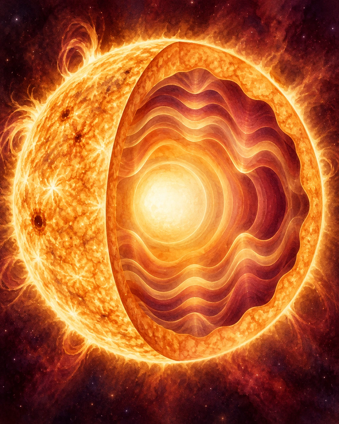
Asteroseismology uses those natural oscillations to investigate stellar interiors. The telescope does not send a probe into the core or record a sound traveling through space. It measures light whose variations are connected to motions inside the star.
The distinction matters whenever an outreach clip invites you to “hear a star.” Such clips can communicate real relationships, but a measurement, an inferred oscillation spectrum and an audible presentation are three different products.
The observation is a long sequence
The Kepler asteroseismology program’s introductory paper describes the demanding requirements: very precise photometry, nearly continuous records over weeks to years, and sampling fast enough for oscillations that can have periods of minutes.
A single accurate brightness measurement cannot recover a frequency. The time sequence is essential. Long observations distinguish nearby frequencies; suitable cadence prevents rapid variation from being sampled misleadingly. Precision, duration and sampling each do a different job.
Imagine two invented rhythms that complete ten and eleven cycles over the same interval. Early on they may look nearly aligned. Continue long enough and their different cycle counts become clear. Shorten the observation and the distinction becomes harder, even if each individual measurement is exact.
This example concerns information in a record, not a recipe for extracting a real stellar spectrum. Actual data contain instrumental effects, noise and other sources of variability. Researchers must distinguish genuine modes from features introduced by the observations themselves.
Frequency and period are reciprocal descriptions
A frequency of one microhertz means one millionth of a cycle per second. The period is one divided by frequency. Therefore 100 microhertz corresponds to 10,000 seconds, or about 2.78 hours.
Use this original three-line exercise before reading a published spectrum:
| Frequency | Period, approximately |
|---|---|
| 100 microhertz | 10,000 seconds |
| 110 microhertz | 9,091 seconds |
| 120 microhertz | 8,333 seconds |
The frequency gaps are equal: ten microhertz each. The period gaps are not. A regular pattern on one axis does not automatically remain regular after taking reciprocals. This is especially useful when two studies discuss frequency spacing and period spacing in different kinds of modes.
These three rows are arithmetic examples, not an observed star or a classification scheme. Their purpose is to make the axes intelligible. Once the units are clear, a plot becomes something you can interrogate instead of a decorative row of peaks.
Different modes sample different physics
Pressure is the principal restoring influence for acoustic, or p, modes. Buoyancy supplies the restoring influence for gravity, or g, modes. The latter name refers to oscillations in a stratified fluid; it does not mean gravitational waves traveling through spacetime.
In red giants, mixed modes can combine gravity-mode behavior in the deep interior with pressure-mode behavior in the outer regions. That connection allows information about the core to appear in observable surface variations.
Bedding and colleagues’ 2011 study used Kepler observations to distinguish red giants burning hydrogen in a shell from those also burning helium in their cores. The useful discriminator was gravity-mode period spacing, accessed through the mode pattern.
In that study, the first population had spacings mostly around fifty seconds, while the helium-burning group had spacings around one hundred to three hundred seconds. Those are differences between modal periods, not a claim that every star brightens once every fifty seconds.
This is a deeper result than measuring a star’s apparent color. Stars with similar outward appearances can occupy different evolutionary stages. The interior-sensitive pattern helps separate histories that surface appearance alone can leave ambiguous.
One well-characterized star and a population are different achievements
JPL’s 2010 account of early Kepler work describes how oscillation analysis constrained an individual evolving star and improved knowledge of stellar properties. This matters for planets as well: an inferred planet size is linked to the properties assigned to its host star.
A later ensemble study by Chaplin and colleagues reported oscillations in five hundred solar-type stars. A sample of that size allowed statistical comparisons with synthetic stellar populations. Its observed mass distribution differed in interesting ways from the model predictions.
That mismatch is useful evidence, not permission to say all stellar evolution calculations failed. A population comparison depends on which stars are observed, which oscillations are detectable and what assumptions enter the synthetic sample. The experiment tests those pieces together.
For a reader, the practical question changes with the scale. For one star, ask which measurements constrain its parameters and how model-dependent they are. For a population, also ask which stars could enter the sample. A beautifully measured subset need not represent every star equally.
Listen to a mapping, with its key supplied
NASA’s Roman asteroseismology feature includes a verified sonification based on simulated data. It starts with the Sun for scale, then moves through progressively larger red giants. The frequencies are sped up into the audible range.
Play it at a comfortable volume, then read its description. The sequence communicates the tendency for larger stars to have slower oscillations and lower corresponding pitches. It is a designed rendering of a simulation, not a microphone recording, and it does not establish that Roman already measured those particular stars.
Try describing the same relationship without sound: a larger oscillating system can take longer to complete a cycle. Then return to the clip and identify which audible change represents that longer timescale. This makes the sonification an explanatory translation with a readable key.
The value of stellar flickering lies in its organized detail. A barely perceptible brightness record can contain several modes, and their relationships constrain a structure no telescope directly resolves. Learning to separate the measured light, the recovered pattern and the modelled interior lets the modest-looking data carry their full scientific weight.
Sources and further exploration
- Gilliland and colleagues: Kepler asteroseismology introduction and first results
- Bedding and colleagues: Gravity-mode spacings distinguish red-giant evolutionary stages
- JPL: Kepler takes the pulse of distant stars
- Chaplin and colleagues: Ensemble asteroseismology of solar-type stars
- NASA: Roman asteroseismology and a simulation-based sonification
Explore all 80 new articles · Browse the complete illustrated collection
Keep exploring at Incoprea.