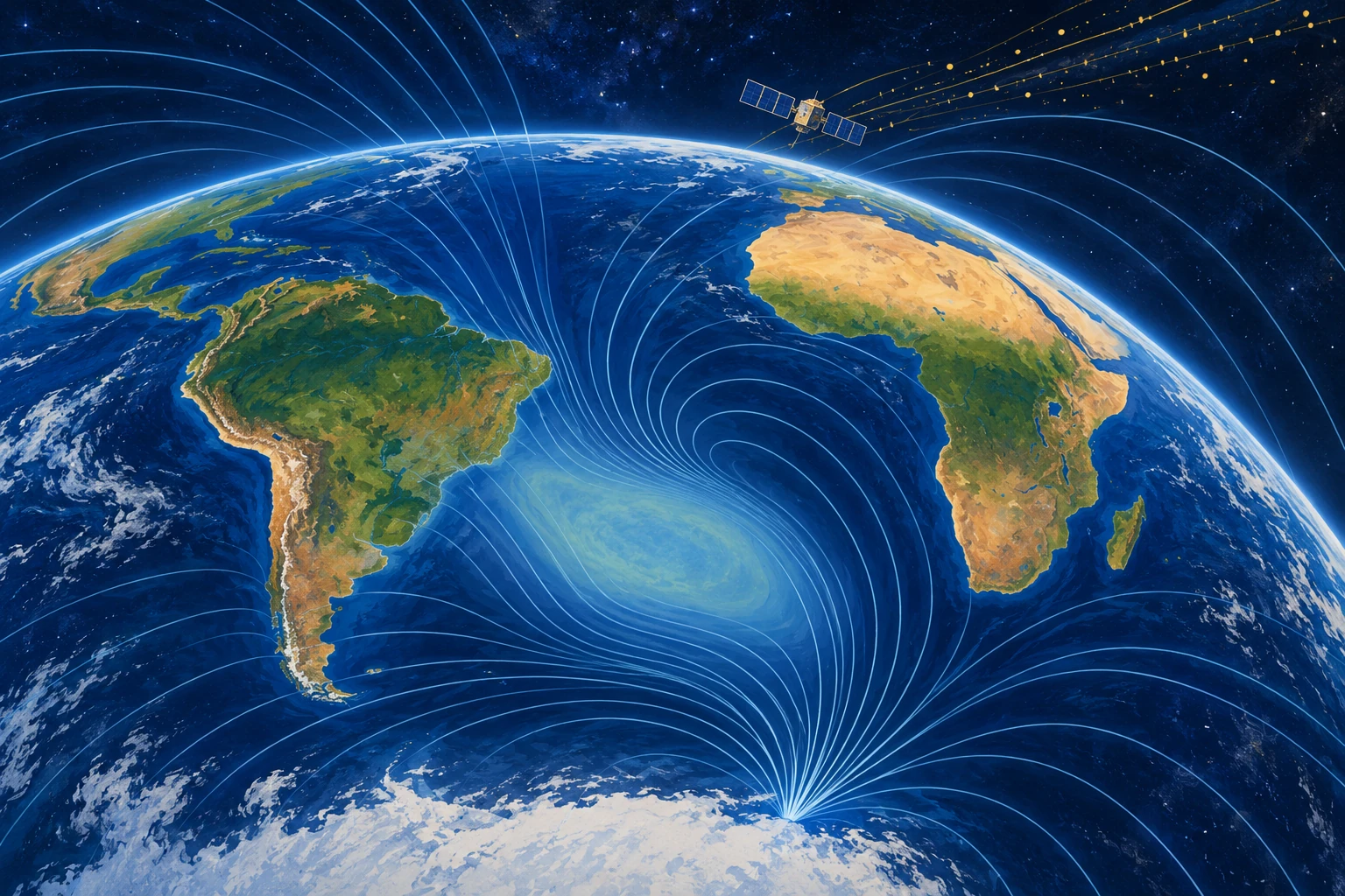
A spacecraft can cross the South Atlantic and encounter a radiation environment that differs markedly from another part of the same orbit. The region is associated with an unusually weak portion of Earth’s magnetic field: the South Atlantic Anomaly, or SAA.
Its name sounds like a mysterious hole. The reality is more specific and more useful. A changing, asymmetric magnetic field alters where trapped energetic particles can reach low orbital altitudes, creating an operational problem for instruments and a scientific clue to processes deep inside Earth.
There is no missing patch of planet
Earth’s field is largely generated by electrically conducting fluid motion in the outer core. It is neither perfectly centered nor a simple permanent bar magnet. Regional features ride on top of a broader dipole-like structure.
NASA’s account of the anomaly connects the weak-field region with the radiation conditions faced by satellites. The “dent” is a metaphor for field geometry and intensity, not a cavity in the atmosphere or a hole through which empty space pours.
Magnetic-field strength and particle flux are related but different quantities. A map of surface field intensity is not automatically a radiation-dose map for a spacecraft at a particular altitude. Orbit, particle energy, detector sensitivity, and time all matter.
The spacecraft consequence is concrete
Energetic particles can disturb electronics, create spurious detector events, degrade components, or interrupt observations. Operators may schedule protective actions or pause sensitive measurements during passages through a hazardous region.
NASA’s ROSAT material provides an example of the anomaly’s relevance to an astronomical mission. An observation gap can therefore reflect an instrument protecting its data or hardware, rather than an absence of interesting objects in the sky.
Imagine a telescope trying to count faint X-ray photons while charged-particle events increase its background. The problem is both reliability and interpretation: which detector signals came from the astronomical target, and which arose from the local environment?
A field that changes in more than one place
ESA’s October 2025 Swarm report describes changes observed between 2014 and 2025, including expansion of the weak-field area and differing behavior toward Africa and South America. The anomaly is not a rigid patch drifting intact across a map.
The report links the behavior to reverse-flux features near the core-mantle boundary. These are inferred aspects of the magnetic field at depth, constrained through observations and modeling. Nobody has placed a camera beside the outer core to film a magnetic patch.
The difference between model inference and direct view matters because a global field model combines several sources. Satellites measure contributions from the core, crust, oceans, ionosphere, and magnetosphere. Separating them requires careful treatment of location, time, and external activity.
What a satellite constellation adds
Multiple spacecraft and ground observatories help constrain spatial structure and temporal change. The CHAOS-7 model paper documents a field model built from several satellite missions and observatory data, then uses it to study the SAA and other changes.
A time sequence is especially valuable. A single map can show a weak region. A consistent series helps estimate how that region evolves and whether different parts behave differently. Data processing must still distinguish a real change from a change in sampling or model construction.
When comparing two published maps, check the altitude, field quantity, color limits, date, and contour threshold. If the colors are rescaled independently, a weak-looking area on one map may not be numerically comparable with the same shade on another.
Draw two maps that answer different questions
For a paper exercise, sketch a surface magnetic-intensity map and a spacecraft radiation-count map. Give each a separate legend. Now ask which map helps investigate the core and which helps an instrument operator plan a passage.
The answer is not exclusive—both can inform both tasks—but the measured quantities differ. Add a second orbit at a different height. Its detector need not record the same counts over the same ground location. This is why “over the anomaly” is incomplete without orbital context.
The exercise is conceptual, not a radiation model. It makes a common visual shortcut visible: a two-dimensional map can hide the three-dimensional environment through which a satellite actually moves.
A forecast is not a photograph from the future
Geomagnetic forecasts combine physical understanding, recent observations, and assumptions about evolution. A graphic that includes projected years should label the boundary between observations and forecast. Otherwise a viewer may treat a modeled future shape as a measurement already made.
That distinction also applies to popular animation. Smoothly moving colors interpolate between states; they do not mean the field was observed continuously at every point. The underlying model and its uncertainty determine what the animation can support.
Make a caption test before sharing an anomaly image: replace “the hole is growing” with the actual plotted quantity, date interval, and threshold. If those details are missing, the picture may still be informative, but its apparent boundary should not be treated as a precisely measured wall. A contour is a selected value in a continuous field.
Does a weak region announce a reversal?
Not by itself. USGS guidance on reversals explains that the geological record contains changing polarity and excursions without a regular reversal timetable. A regional anomaly is not sufficient evidence for a dated prediction of a global transition.
It is equally unhelpful to describe the field as either perfectly protective or completely absent. The magnetosphere and atmosphere have different roles, and the SAA’s practical concern is especially clear for spacecraft. A sensational ground-level catastrophe does not follow from an operational satellite hazard.
The useful anomaly
Read an actual mission description and look for its measurement altitude, detector type, and data-screening rules. Then return to the field map. The connection between them becomes more concrete than a frightening red circle.
The SAA is compelling because one regional pattern connects a telescope’s noisy detector, the motion of charged particles, and liquid-metal processes thousands of kilometers below our feet. It becomes more interesting as those links become more precise.
Sources and a next step
- NASA: tracking the South Atlantic Anomaly
- NASA HEASARC: ROSAT and the SAA
- ESA 2025: Swarm observations of the changing anomaly
- Finlay et al.: CHAOS-7 geomagnetic field model
- USGS: reversals and the geological record
Continue exploring art, ideas, and unexpected connections at Incoprea.